Kolmogorov-Smirnov (Lilliefors) test
The Kolmogorov-Smirnov test measures the largest vertical distance between the empirical cumulative distribution function of a sample and a reference CDF. The Lilliefors variant adjusts the critical values for the case where the distribution parameters are estimated from the data, which is always the case when testing for normality.
KS test vs Lilliefors test
The two tests share the same statistic but differ in how the reference distribution is specified:
- KS test: the reference distribution is fully specified (known parameters). For example, testing whether data follow a \(N(10, 4)\) with \(\mu=10\) and \(\sigma=2\) fixed in advance.
- Lilliefors test: the parameters are estimated from the data (\(\hat{\mu} = \bar{x}\), \(\hat{\sigma} = S\)). This is what you do when testing for normality without knowing \(\mu\) and \(\sigma\). Estimating parameters from the data makes the test statistic stochastically smaller, so the KS critical values are too conservative: Lilliefors recomputed them via simulation.
In practice, when you say “KS test for normality,” you almost always mean the Lilliefors test.
Test statistic
\[D = \max_x \left| F_n(x) - F_0(x) \right|\]
where \(F_n(x)\) is the empirical CDF of the sample and \(F_0(x)\) is the reference CDF (normal with estimated parameters in the Lilliefors case). The larger \(D\) is, the more the sample deviates from the reference distribution.
Hypotheses: \(H_0\): the data follow the specified distribution. \(H_1\): they do not.
The p-value is computed by comparing \(D\) to the Lilliefors distribution (via simulation or dedicated tables), not the standard KS distribution.
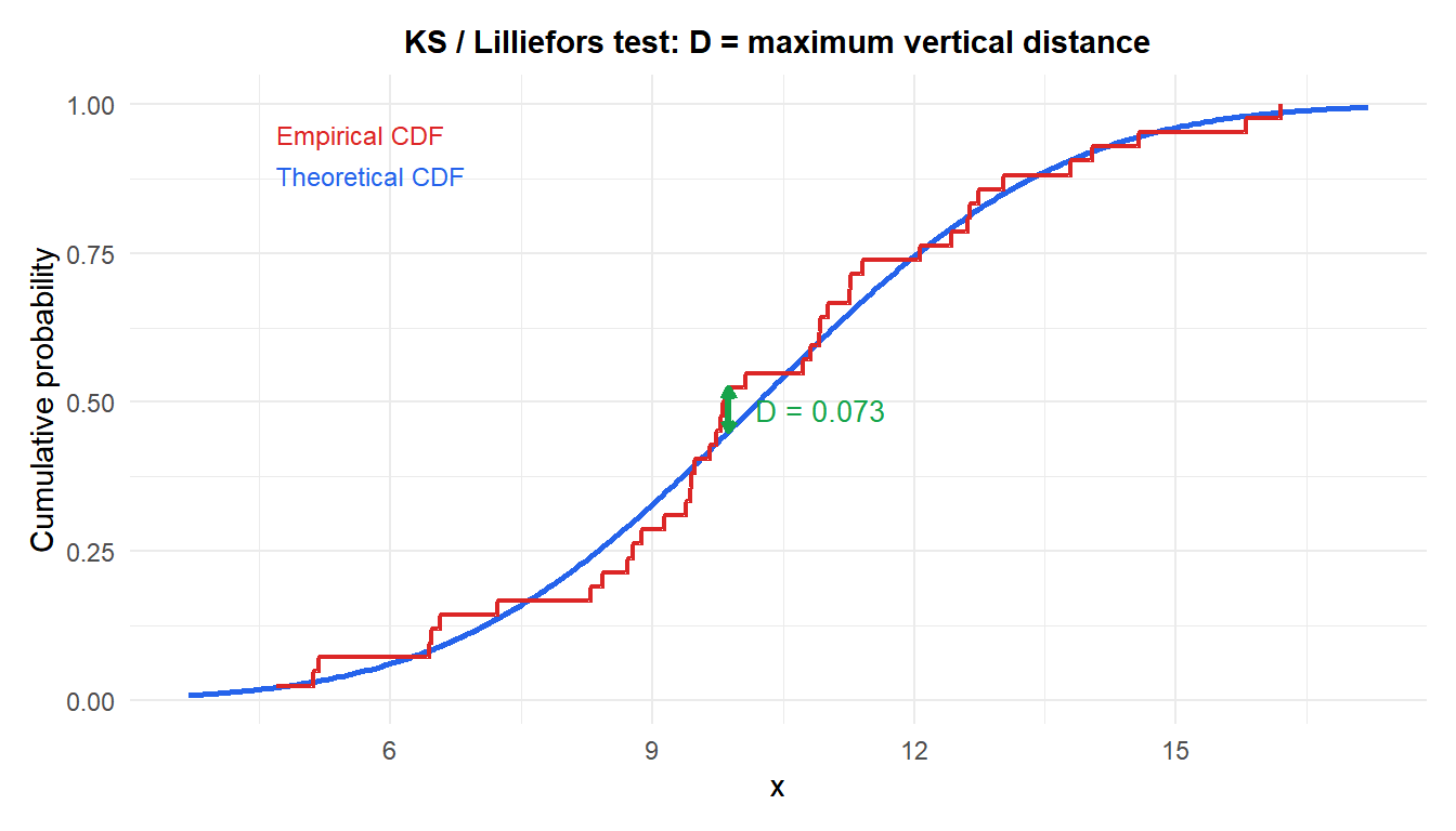
The red step function is the empirical CDF; the blue curve is the theoretical normal CDF with estimated parameters. The green segment marks the maximum distance \(D\).
Step-by-step example
A lab measures the viscosity of 30 samples. Before applying a \(t\)-test, the analyst checks for normality. The data give \(\bar{x} = 12.4\) cP, \(S = 1.8\) cP.
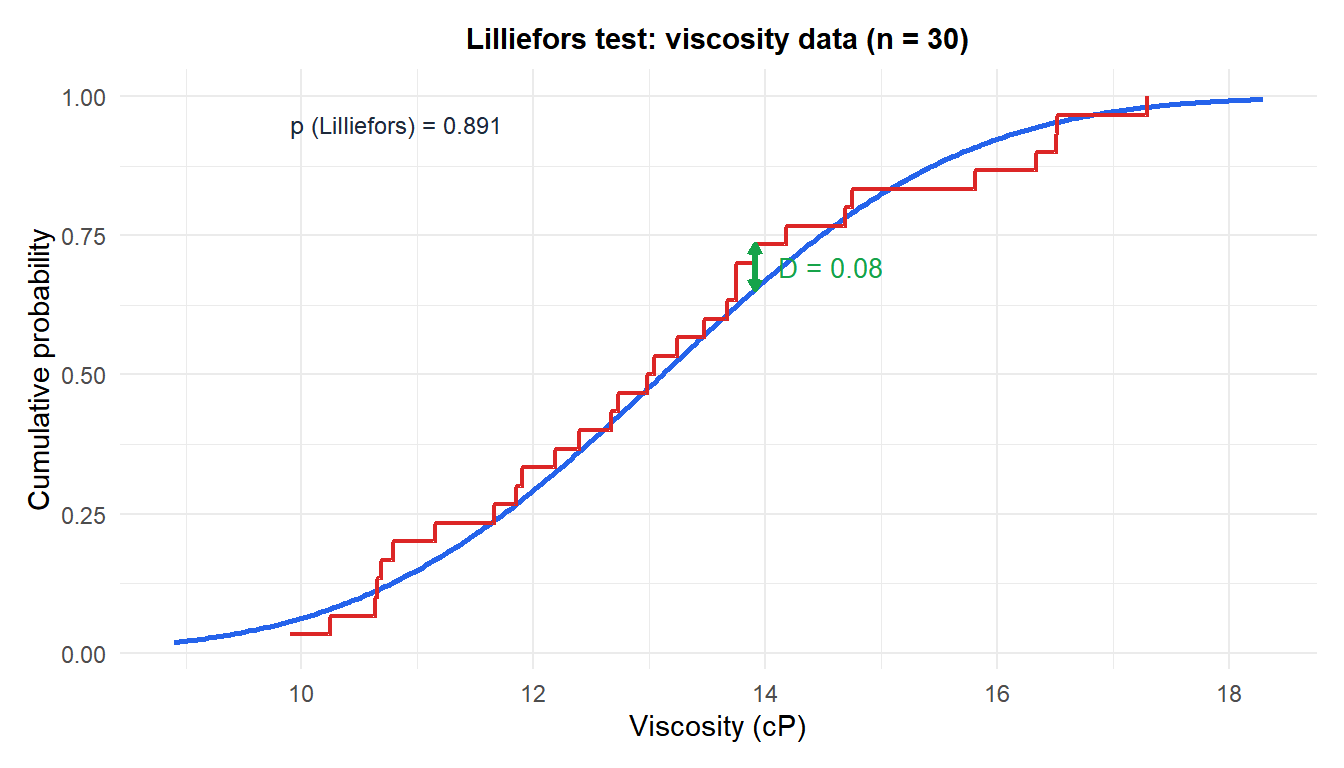
If \(p > 0.05\), normality is not rejected and the \(t\)-test can proceed. In R:
library(nortest)
lillie.test(x)   # Lilliefors test
ks.test(x, "pnorm", mean(x), sd(x))  # KS test (wrong for normality: use lillie.test)
Comparison with other normality tests
The KS/Lilliefors test is one of several options for testing normality. Each has different strengths:
| Test | Best for | Power | Notes |
|---|---|---|---|
| Lilliefors | General normality | Moderate | Parameters estimated from data |
| Shapiro-Wilk | Small to medium samples (\(n \leq 50\)) | High | Most powerful for normality |
| Anderson-Darling | Tail sensitivity | High | Weights tails more than center |
| KS (original) | Known parameters | Moderate | Too conservative when parameters estimated |
⚠️ Shapiro-Wilk is almost always preferred over Lilliefors for normality testing
For testing normality, Shapiro-Wilk has higher power than the Lilliefors test across almost all sample sizes and departures from normality. Unless you have a specific reason to use Lilliefors (e.g., software constraints), use Shapiro-Wilk in R: shapiro.test(x).
The original KS test (with known parameters) should never be used for normality testing when the mean and variance are estimated from the data: the p-values will be too large (too conservative) because the KS critical values assume fully specified distributions.
⚠️ All normality tests have low power for small samples and high power for large ones
For \(n < 20\), normality tests rarely reject \(H_0\) even for clearly non-normal data: the test has low power. For \(n > 100\), they often reject \(H_0\) for trivial departures from normality that have no practical consequence. A Q-Q plot is always a useful complement to the formal test: it shows where and how the data depart from normality, which the p-value alone does not reveal.
💡 Practical workflow for normality checking
A robust approach to normality checking before parametric tests:
- Plot a Q-Q plot:
qqnorm(x); qqline(x). - Run Shapiro-Wilk:
shapiro.test(x). - If \(n > 50\), complement with Anderson-Darling:
nortest::ad.test(x). - Consider the robustness of the downstream test: the \(t\)-test is fairly robust to mild non-normality for \(n \geq 30\), so a minor departure from normality may not matter.
Reject the parametric test only when the Q-Q plot shows a clear systematic departure and the normality test confirms it.

