Hypothesis testing for a proportion
The one-sample z-test for a proportion evaluates whether a population proportion equals a specific hypothesized value. It relies on the normal approximation to the binomial, which requires checking that the sample is large enough before applying the test.
Hypotheses
| Test | \(H_0\) | \(H_1\) |
|---|---|---|
| Two-sided | \(p = p_0\) | \(p \neq p_0\) |
| One-sided right | \(p = p_0\) | \(p > p_0\) |
| One-sided left | \(p = p_0\) | \(p < p_0\) |
Test statistic
Given \(x\) successes in \(n\) trials, \(\hat{p} = x/n\). The test statistic is:
\[Z = \frac{\hat{p} - p_0}{\sqrt{p_0(1-p_0)/n}}\]
Under \(H_0\), \(Z\) follows a standard normal distribution. Note that the denominator uses \(p_0\), not \(\hat{p}\): we compute the standard error under the null hypothesis, not under the observed proportion.
The normal approximation is valid when both:
\[n p_0 \geq 10 \quad \text{and} \quad n(1-p_0) \geq 10\]
⚠️ When the normal approximation fails, use exact methods
When \(np_0 < 10\) or \(n(1-p_0) < 10\) (rare events, small samples, or extreme proportions), the binomial distribution is skewed and the normal approximation is unreliable. In those cases:
- Use the exact binomial test:
binom.test()in R. It computes the exact p-value from the binomial distribution. - For confidence intervals, use the Wilson score interval rather than the Wald interval.
The condition \(np_0 \geq 10\) (not \(\geq 5\), as older textbooks state) is the current recommended threshold for the normal approximation.
Examples
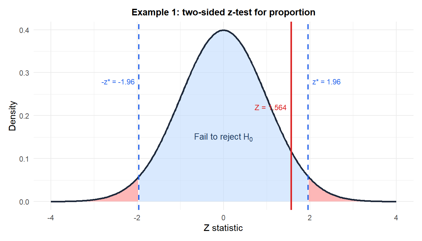
Example 1: defect rate in manufacturing (two-sided)
A production line has a historical defect rate of \(p_0 = 0.08\). After a process change, a quality engineer inspects 200 units and finds 22 defective (\(\hat{p} = 0.110\)). Has the defect rate changed?
Check conditions: \(np_0 = 200 \times 0.08 = 16 \geq 10\) and \(n(1-p_0) = 184 \geq 10\). Normal approximation is valid.
Hypotheses: \(H_0: p = 0.08\) vs \(H_1: p \neq 0.08\).
Test statistic:
\[Z = \frac{0.110 - 0.08}{\sqrt{0.08 \times 0.92 / 200}} = \frac{0.030}{\sqrt{0.000368}} = \frac{0.030}{0.01918} \approx 1.564\]
p-value (two-sided):
\[p = 2 \times P(Z \geq 1.564) = 2 \times 0.059 = 0.118\]
Decision: \(p = 0.118 > 0.05\), fail to reject \(H_0\).
The observed increase from 8% to 11% defects is not statistically significant at the 5% level. However, the sample size may be insufficient to detect a change of this magnitude reliably. Power analysis would be warranted before concluding no change occurred.
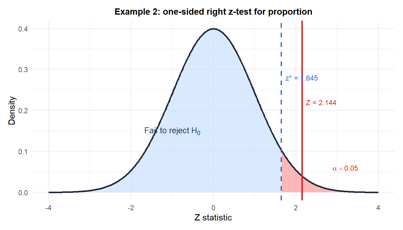
Example 2: conversion rate improvement (one-sided right)
An e-commerce platform’s current checkout conversion rate is \(p_0 = 0.32\). After a redesign, 148 out of 400 users complete a purchase (\(\hat{p} = 0.370\)). Is there evidence the redesign improved the conversion rate?
Check conditions: \(np_0 = 400 \times 0.32 = 128 \geq 10\) and \(n(1-p_0) = 272 \geq 10\). Normal approximation is valid.
Hypotheses: \(H_0: p = 0.32\) vs \(H_1: p > 0.32\).
Test statistic:
\[Z = \frac{0.370 - 0.32}{\sqrt{0.32 \times 0.68 / 400}} = \frac{0.050}{\sqrt{0.000544}} = \frac{0.050}{0.02333} \approx 2.144\]
p-value (one-sided right):
\[p = P(Z \geq 2.144) \approx 0.016\]
Decision: \(p = 0.016 < 0.05\), reject \(H_0\).
There is significant evidence at the 5% level that the redesign improved the conversion rate. The conversion rate increased by approximately 5 percentage points, a relative improvement of about 16%.
Running the test in R
# Example 1: two-sided
prop.test(x = 22, n = 200, p = 0.08, alternative = "two.sided", correct = FALSE)

# Example 2: one-sided right
prop.test(x = 148, n = 400, p = 0.32, alternative = "greater", correct = FALSE)

# Exact binomial test (for small samples)
binom.test(x = 22, n = 200, p = 0.08, alternative = "two.sided")
prop.test() uses the chi-squared approximation (equivalent to the z-test). correct = FALSE disables the Yates continuity correction, which is rarely needed with large samples.
💡 Interpreting the result
A significant result means the data are inconsistent with \(H_0: p = p_0\). Always report the effect size alongside the p-value: the difference \(\hat{p} - p_0\) and its confidence interval convey both statistical significance and practical importance. A change from 8% to 11% defects might be statistically non-significant with \(n=200\) but practically important; with \(n=2000\) it would be highly significant.

