Chi-square test
The chi-square test is the standard method for analyzing categorical data. It comes in two forms: the test of independence (are two categorical variables associated?) and the goodness-of-fit test (does a categorical variable follow a specific distribution?). Both use the same test statistic and the chi-squared distribution as the reference.
The chi-square statistic
Both tests use the same core idea: compare observed frequencies \(O_i\) to expected frequencies \(E_i\) under \(H_0\).
\[\chi^2 = \sum \frac{(O_i - E_i)^2}{E_i}\]
Large values of \(\chi^2\) indicate that the observed data are far from what \(H_0\) predicts. Under \(H_0\), this statistic follows a \(\chi^2\) distribution whose degrees of freedom depend on the type of test.
Test of independence
Used to test whether two categorical variables are associated in a contingency table.
Hypotheses: \(H_0\): the two variables are independent. \(H_1\): there is an association.
Expected frequencies for each cell \((i, j)\):
\[E_{ij} = \frac{\text{row total}_i \times \text{column total}_j}{\text{grand total}}\]
Degrees of freedom: \(df = (r-1)(c-1)\), where \(r\) = number of rows and \(c\) = number of columns.
A survey of 200 people records gender (Male/Female) and product preference (Like/Dislike):
| Like | Dislike | Total | |
|---|---|---|---|
| Male | 60 | 40 | 100 |
| Female | 30 | 70 | 100 |
| Total | 90 | 110 | 200 |
Expected frequencies under independence:
\[E_{11} = \frac{100 \times 90}{200} = 45, \quad E_{12} = \frac{100 \times 110}{200} = 55\] \[E_{21} = \frac{100 \times 90}{200} = 45, \quad E_{22} = \frac{100 \times 110}{200} = 55\]
Test statistic:
\[\chi^2 = \frac{(60-45)^2}{45} + \frac{(40-55)^2}{55} + \frac{(30-45)^2}{45} + \frac{(70-55)^2}{55}\] \[= 5.000 + 4.091 + 5.000 + 4.091 = 18.182\]
\(df = (2-1)(2-1) = 1\). Critical value at \(\alpha=0.05\): \(\chi^2_{0.05,1} = 3.841\).
Since \(18.182 > 3.841\), reject \(H_0\). There is a significant association between gender and product preference.
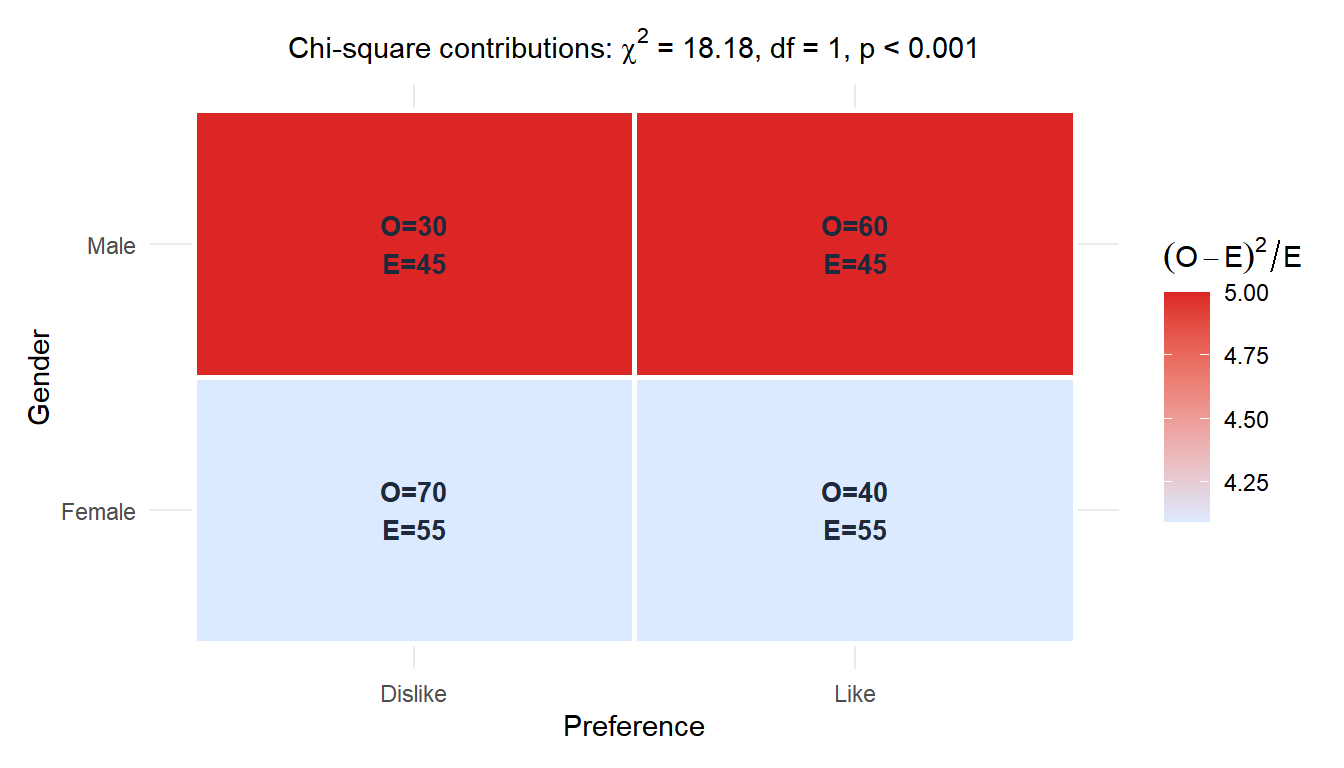
The heatmap shows each cell’s contribution to \(\chi^2\): red cells deviate most from independence.
Effect size: Cramér’s V
The p-value tells you whether the association is significant, not how strong it is. For contingency tables, use Cramér’s V:
\[V = \sqrt{\frac{\chi^2}{n \times \min(r-1, c-1)}}\]
\(V\) ranges from 0 (no association) to 1 (perfect association). For a \(2 \times 2\) table it equals the absolute value of the phi coefficient.
For the example: \(V = \sqrt{18.182 / (200 \times 1)} = \sqrt{0.0909} \approx 0.301\). A moderate association.
⚠️ Statistical significance is not the same as strong association
With large samples, even trivial associations produce significant chi-square statistics. A survey of 10,000 people might find \(\chi^2 = 5.2\) (\(p = 0.023\)) for an association with \(V = 0.02\): statistically significant but practically negligible.
Always report Cramér’s V alongside the p-value. As a rough guide: \(V < 0.1\) is weak, \(0.1 \leq V < 0.3\) is moderate, \(V \geq 0.3\) is strong.
Goodness-of-fit test
Used to test whether a single categorical variable follows a specific distribution.
Hypotheses: \(H_0\): the variable follows the specified distribution. \(H_1\): it does not.
Degrees of freedom: \(df = k - 1\), where \(k\) is the number of categories.
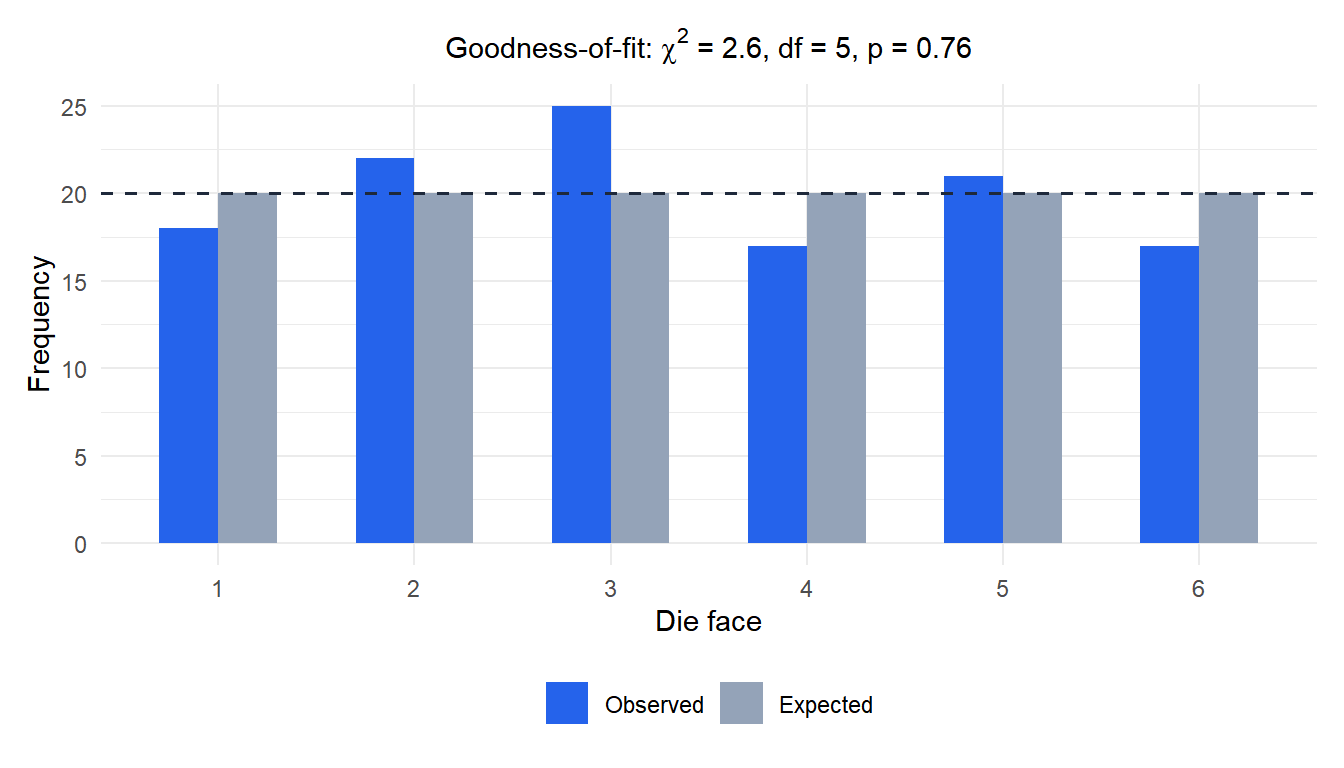
A die is rolled 120 times. If fair, each face should appear 20 times. Observed counts:
| Face | 1 | 2 | 3 | 4 | 5 | 6 |
|---|---|---|---|---|---|---|
| Observed | 18 | 22 | 25 | 17 | 21 | 17 |
| Expected | 20 | 20 | 20 | 20 | 20 | 20 |
\[\chi^2 = \frac{(18-20)^2}{20} + \frac{(22-20)^2}{20} + \frac{(25-20)^2}{20} + \frac{(17-20)^2}{20} + \frac{(21-20)^2}{20} + \frac{(17-20)^2}{20}\] \[= 0.2 + 0.2 + 1.25 + 0.45 + 0.05 + 0.45 = 2.6\]
\(df = 6 - 1 = 5\). Critical value at \(\alpha=0.05\): \(\chi^2_{0.05,5} = 11.07\).
Since \(2.6 < 11.07\), fail to reject \(H_0\). No significant evidence that the die is unfair.
Assumptions
Both chi-square tests require:
- Independence: observations are not paired or clustered.
- Expected frequencies \(\geq 5\): each cell in the table should have an expected frequency of at least 5. If this is violated, merge categories or use Fisher’s exact test (for \(2 \times 2\) tables).
- Counts, not percentages: the test statistic must be computed from raw counts, not proportions.
⚠️ Chi-square tests do not identify which cells drive the association
A significant result in a large contingency table tells you there is an association somewhere, but not where. Use standardized residuals to identify which cells deviate most from independence:
\[r_{ij} = \frac{O_{ij} - E_{ij}}{\sqrt{E_{ij}}}\]
Cells with \(|r_{ij}| > 2\) are contributing significantly to the overall \(\chi^2\). In R: chisq.test(table)$residuals.
Running the tests in R
Both tests are available in base R. For the test of independence, pass the contingency table to chisq.test(). For goodness-of-fit, pass the observed counts and optionally the expected probabilities. The correct = FALSE argument disables the Yates continuity correction, which is rarely needed with large samples but is applied by default for \(2 \times 2\) tables.
# Test of independence
table_data <- matrix(c(60, 40, 30, 70), nrow = 2)
chisq.test(table_data, correct = FALSE)

# Cramér's V (package rstatix or vcd)
library(vcd)
assocstats(table_data)

# Goodness-of-fit
observed <- c(18, 22, 25, 17, 21, 17)
chisq.test(observed)  # tests against uniform by default
The output includes the test statistic, degrees of freedom, and p-value. Standardized residuals are accessible via chisq.test(table_data)$residuals, which helps identify which cells drive a significant result.
💡 Choosing between chi-square and Fisher's exact test
For \(2 \times 2\) tables with small samples (any expected frequency \(< 5\)), use Fisher’s exact test (fisher.test() in R). It computes the exact p-value from the hypergeometric distribution and does not require large samples. For larger tables, chi-square is the standard approach.

