Analysis of variance (ANOVA)
One-way ANOVA tests whether the means of three or more independent groups are all equal. It extends the two-sample t-test to multiple groups while controlling the Type I error rate, which would inflate if multiple t-tests were applied pairwise.
Why not multiple t-tests?
With \(k\) groups, there are \(\binom{k}{2}\) possible pairwise comparisons. At \(\alpha = 0.05\), each t-test has a 5% chance of a false positive. With 3 groups (3 comparisons), the probability of at least one false positive is \(1 - 0.95^3 \approx 0.14\): nearly three times the nominal rate. ANOVA tests all groups simultaneously with a single F-statistic, keeping the Type I error at \(\alpha\).
Hypotheses
\[H_0: \mu_1 = \mu_2 = \cdots = \mu_k \qquad H_1: \text{at least one } \mu_i \neq \mu_j\]
A significant result only tells you that at least one group mean differs. Post-hoc tests identify which pairs differ.
Partitioning variance
ANOVA decomposes the total variation into two components:
\[SS_\text{total} = SS_\text{between} + SS_\text{within}\]
where:
- \(SS_\text{between} = \sum_{i=1}^k n_i (\bar{y}_i - \bar{y})^2\): variation due to differences between group means.
- \(SS_\text{within} = \sum_{i=1}^k \sum_{j=1}^{n_i} (y_{ij} - \bar{y}_i)^2\): variation within groups (residual).
The F-statistic is the ratio of mean squares:
\[F = \frac{MS_\text{between}}{MS_\text{within}} = \frac{SS_\text{between}/(k-1)}{SS_\text{within}/(N-k)}\]
Under \(H_0\) and the normality assumption, \(F \sim F(k-1, N-k)\). Large \(F\) values indicate that between-group variation exceeds what would be expected from random sampling alone.
The ANOVA table
Results are typically presented in a standardized table:
| Source | SS | df | MS | F | p-value |
|---|---|---|---|---|---|
| Between groups | \(SS_B\) | \(k-1\) | \(MS_B = SS_B/(k-1)\) | \(F = MS_B/MS_W\) | \(P(F_{k-1,N-k} \geq F)\) |
| Within groups | \(SS_W\) | \(N-k\) | \(MS_W = SS_W/(N-k)\) | ||
| Total | \(SS_T\) | \(N-1\) |
Complete example: three diet plans
A nutritionist compares weight loss (kg) across three diet plans after 8 weeks:
- Diet A: 4, 5, 6, 5, 7 (\(n_1 = 5\), \(\bar{y}_1 = 5.4\))
- Diet B: 8, 7, 9, 10, 8 (\(n_2 = 5\), \(\bar{y}_2 = 8.4\))
- Diet C: 3, 2, 4, 3, 2 (\(n_3 = 5\), \(\bar{y}_3 = 2.8\))
Overall mean: \(\bar{y} = (5.4 + 8.4 + 2.8)/3 = 5.533\).
\(SS_\text{between}\):
\[SS_B = 5(5.4-5.533)^2 + 5(8.4-5.533)^2 + 5(2.8-5.533)^2\] \[= 5(0.018) + 5(8.211) + 5(7.474) = 0.089 + 41.056 + 37.369 = 78.533\]
\(SS_\text{within}\) (sum of squared deviations within each group):
Diet A: \((4-5.4)^2+(5-5.4)^2+(6-5.4)^2+(5-5.4)^2+(7-5.4)^2 = 1.96+0.16+0.36+0.16+2.56 = 5.2\)
Diet B: \((8-8.4)^2+(7-8.4)^2+(9-8.4)^2+(10-8.4)^2+(8-8.4)^2 = 0.16+1.96+0.36+2.56+0.16 = 5.2\)
Diet C: \((3-2.8)^2+(2-2.8)^2+(4-2.8)^2+(3-2.8)^2+(2-2.8)^2 = 0.04+0.64+1.44+0.04+0.64 = 2.8\)
\(SS_W = 5.2 + 5.2 + 2.8 = 13.2\)
ANOVA table:
| Source | SS | df | MS | F | p-value |
|---|---|---|---|---|---|
| Between | 78.533 | 2 | 39.267 | 35.70 | < 0.001 |
| Within | 13.200 | 12 | 1.100 | ||
| Total | 91.733 | 14 |
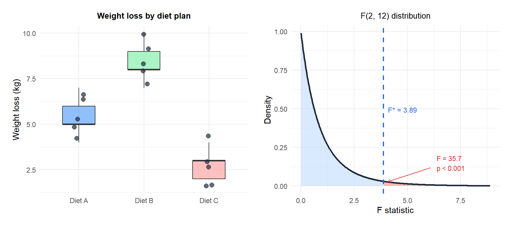
Decision: \(F = 35.70 \gg F_{0.05,2,12} = 3.885\), \(p < 0.001\). Reject \(H_0\): at least one diet produces different mean weight loss.
Post-hoc tests: which groups differ?
ANOVA’s rejection of \(H_0\) only says some means differ. Post-hoc tests identify which pairs, while controlling for multiple comparisons.
Tukey’s HSD (Honestly Significant Difference) is the standard choice when comparing all pairs. It uses the studentized range distribution and controls the familywise error rate at \(\alpha\).
For equal group sizes, the minimum significant difference between two means is:
\[\text{HSD} = q_{\alpha,k,N-k} \sqrt{\frac{MS_W}{n}}\]
where \(q_{\alpha,k,N-k}\) is the critical value from the studentized range distribution.
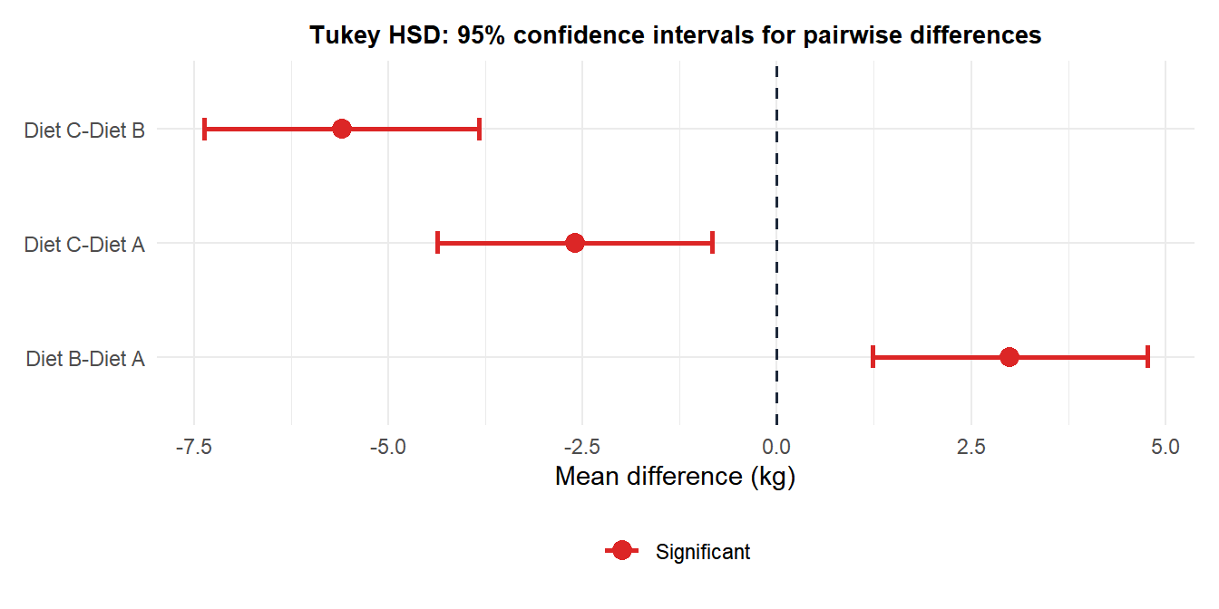
All three pairwise comparisons are significant: all diets differ from each other. Diet B produces the most weight loss; Diet C the least.
Assumptions
One-way ANOVA requires:
- Independence: observations are independent within and across groups.
- Normality: residuals are approximately normal within each group. Check with Shapiro-Wilk or Q-Q plots.
- Homoscedasticity: equal variances across groups. Check with Levene’s test.
⚠️ ANOVA is robust to mild normality violations but not to heteroscedasticity
For equal or similar sample sizes, ANOVA is fairly robust to mild non-normality (CLT). It is more sensitive to unequal variances, especially when group sizes differ.
If Levene’s test rejects homoscedasticity:
- Use Welch’s ANOVA (
oneway.test(..., var.equal = FALSE)in R): does not assume equal variances. - Use Kruskal-Wallis as a nonparametric alternative.
If normality is severely violated: use Kruskal-Wallis.
Running ANOVA in R
# One-way ANOVA
fit <- aov(loss ~ diet, data = df_diet)
summary(fit)

# Welch's ANOVA (unequal variances)
oneway.test(loss ~ diet, data = df_diet, var.equal = FALSE)

# Tukey post-hoc
TukeyHSD(fit)

# Levene's test for homoscedasticity
car::leveneTest(loss ~ diet, data = df_diet)

# Kruskal-Wallis (nonparametric alternative)
kruskal.test(loss ~ diet, data = df_diet)
💡 ANOVA vs multiple t-tests: the key rule
Never run pairwise t-tests as a substitute for ANOVA. Use ANOVA first to test the global \(H_0\). If significant, use post-hoc tests (Tukey, Bonferroni, Scheffé) that control the familywise error rate. Running raw pairwise t-tests inflates the Type I error rate and is not scientifically valid.

