Estimation of a proportion
The sample proportion \(\hat{p}\) is the standard point estimator for a population proportion \(p\). It is unbiased, consistent, and approximately normal for large samples, making it the foundation of all inference about proportions.
Definition
The population proportion \(p\) is the fraction of a population that has a given characteristic. Since we cannot measure the entire population, we take a random sample of size \(n\) and count the number of successes \(X\).
The sample proportion is:
\[\hat{p} = \frac{X}{n}\]
where \(X \sim \text{Binomial}(n, p)\). Since \(E[X] = np\), the sample proportion is an unbiased estimator: \(E[\hat{p}] = p\).
Sampling distribution of \(\hat{p}\)
Before collecting data, \(\hat{p}\) is a random variable. Its exact distribution is:
\[\hat{p} = X/n \quad \text{where } X \sim \text{Binomial}(n, p)\]
By the Central Limit Theorem, for large enough \(n\):
\[\hat{p} \approx N\!\left(p,\ \sqrt{\frac{p(1-p)}{n}}\right)\]
The standard error of \(\hat{p}\) is:
\[\text{SE}(\hat{p}) = \sqrt{\frac{p(1-p)}{n}}\]
Since \(p\) is unknown, it is estimated by \(\hat{p}\) in practice:
\[\widehat{\text{SE}}(\hat{p}) = \sqrt{\frac{\hat{p}(1-\hat{p})}{n}}\]
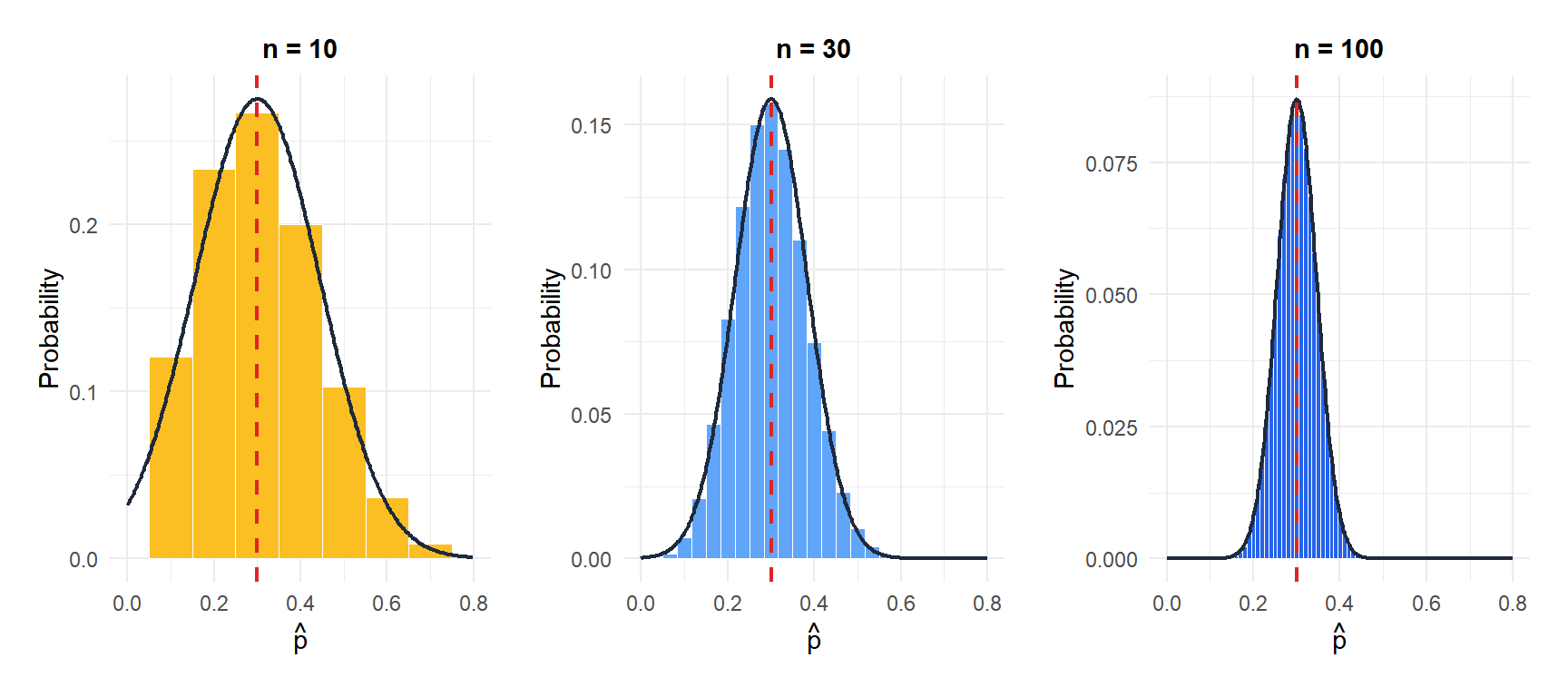
For small \(n\), the discrete binomial distribution is clearly not normal (especially for \(p\) near 0 or 1). As \(n\) grows, the normal approximation (black curve) fits closely.
Standard error and precision
The standard error \(\text{SE}(\hat{p}) = \sqrt{p(1-p)/n}\) depends on both the true proportion and the sample size.
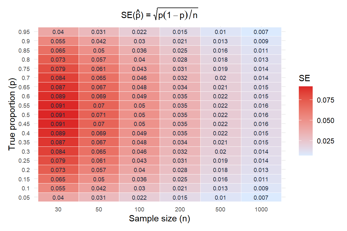
Key observations:
- SE is maximized at \(p = 0.5\) (most uncertain case) and decreases toward 0 and 1.
- For \(p = 0.5\) and \(n = 100\): \(\text{SE} = \sqrt{0.25/100} = 0.05\).
- To halve the SE, you need four times the sample size.
When is the normal approximation valid?
The standard rule of thumb requires both:
\[n\hat{p} \geq 10 \quad \text{and} \quad n(1-\hat{p}) \geq 10\]
This ensures enough successes and failures for the binomial to be well-approximated by a normal distribution.
⚠️ The normal approximation fails for rare events and small samples
When \(p\) is very small (rare events) or very large, or when \(n\) is small, the normal approximation is poor:
- For \(p = 0.02\) and \(n = 100\): \(n\hat{p} = 2 < 10\). The distribution is strongly right-skewed and the normal approximation is invalid.
- In this case, use the exact binomial distribution or, for rare events, the Poisson approximation.
A more conservative alternative is the Wilson score interval, which performs well even when the normal approximation fails, and is preferred in many applied settings over the standard Wald interval.
Examples
Quality control: defect rate
A factory inspects 200 components and finds 14 defective. The point estimate of the defect rate is:
\[\hat{p} = \frac{14}{200} = 0.07\]
The estimated standard error:
\[\widehat{\text{SE}} = \sqrt{\frac{0.07 \times 0.93}{200}} = \sqrt{\frac{0.0651}{200}} \approx 0.018\]
Check: \(n\hat{p} = 200 \times 0.07 = 14 \geq 10\) and \(n(1-\hat{p}) = 186 \geq 10\). The normal approximation is valid.
The best estimate of the population defect rate is 7%, with a standard error of 1.8%.
Clinical trial: response rate
In a phase II trial, 45 out of 120 patients respond to a new treatment:
\[\hat{p} = \frac{45}{120} = 0.375\]
\[\widehat{\text{SE}} = \sqrt{\frac{0.375 \times 0.625}{120}} \approx \sqrt{0.001953} \approx 0.044\]
The point estimate of the response rate is 37.5% with a standard error of 4.4%.
Same \(\hat{p} = 0.375\), different sample sizes:
| \(n\) | \(\widehat{\text{SE}}\) | Margin of error (\(\times 1.96\)) |
|---|---|---|
| 30 | 0.088 | ±17.3% |
| 120 | 0.044 | ±8.7% |
| 480 | 0.022 | ±4.3% |
| 1920 | 0.011 | ±2.2% |
Quadrupling the sample size halves the margin of error. To achieve a margin of error of 2%, you need roughly 2,000 observations when \(p \approx 0.375\).
💡 Choosing between estimators for proportions
- Standard \(\hat{p} = X/n\): the default, unbiased, works well when \(n\hat{p} \geq 10\) and \(n(1-\hat{p}) \geq 10\).
- Add-2 estimator (Agresti-Coull): \(\tilde{p} = (X+2)/(n+4)\). Slightly biased but performs better for small \(n\) or extreme \(p\). Recommended for confidence intervals.
- Bayesian estimator: uses a Beta prior. For a uniform prior Beta(1,1), the posterior mean is \((X+1)/(n+2)\), a natural smoothing toward 0.5.
For large samples with \(p\) not too extreme, all three give nearly identical results.

