Confidence interval for the difference between two proportions
The confidence interval for \(p_1 - p_2\) estimates the range of plausible values for the true difference between two population proportions. It is the standard tool for comparing conversion rates, response rates, or any binary outcome between two independent groups.
Formula
Given two independent samples with \(x_1\) successes in \(n_1\) trials and \(x_2\) successes in \(n_2\) trials, the sample proportions are \(\hat{p}_1 = x_1/n_1\) and \(\hat{p}_2 = x_2/n_2\).
A \((1-\alpha)\) CI for \(p_1 - p_2\) is:
\[(\hat{p}_1 - \hat{p}_2) \pm z_{\alpha/2} \sqrt{\frac{\hat{p}_1(1-\hat{p}_1)}{n_1} + \frac{\hat{p}_2(1-\hat{p}_2)}{n_2}}\]
The standard error of the difference uses the individual SEs combined in quadrature (square root of the sum of variances), since the two samples are independent.
The normal approximation is valid when all four counts are at least 10:
\[n_1\hat{p}_1 \geq 10, \quad n_1(1-\hat{p}_1) \geq 10, \quad n_2\hat{p}_2 \geq 10, \quad n_2(1-\hat{p}_2) \geq 10\]
⚠️ When the normal approximation fails
When any of the four counts is below 10, the normal approximation is unreliable. In that case:
- Use Fisher’s exact test for a hypothesis test.
- Use the Newcombe interval (based on Wilson score intervals for each proportion separately), which maintains better coverage without requiring large samples.
- For very rare events, consider the Poisson approximation.
The same condition that validates the individual proportion CI must hold for both groups to validate the difference CI.
Sampling distribution of the difference
By independence and the CLT, \(\hat{p}_1 - \hat{p}_2\) is approximately normal with:
\[E[\hat{p}_1 - \hat{p}_2] = p_1 - p_2\]
\[\text{SE}(\hat{p}_1 - \hat{p}_2) = \sqrt{\frac{p_1(1-p_1)}{n_1} + \frac{p_2(1-p_2)}{n_2}}\]
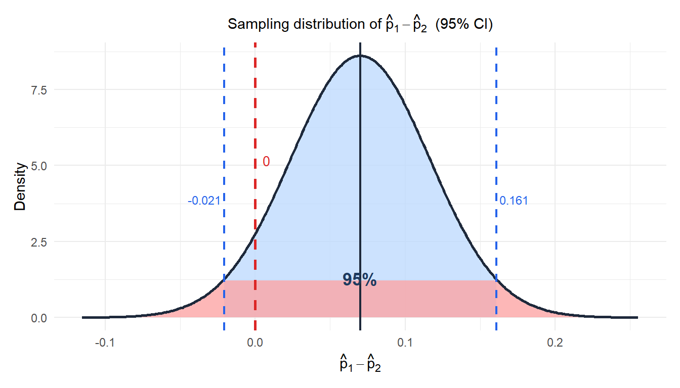
The red dashed line at 0 represents “no difference”. Since 0 falls outside the CI, the difference is statistically significant at the 5% level.
Step-by-step examples
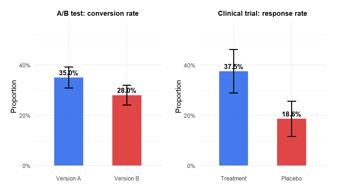
Example 1: A/B testing
An e-commerce platform tests two landing page designs. Version A is shown to 500 visitors, 175 of whom make a purchase. Version B is shown to 500 visitors, 140 of whom make a purchase.
\[\hat{p}_A = 175/500 = 0.350, \qquad \hat{p}_B = 140/500 = 0.280\]
Check conditions:
\[n_A\hat{p}_A = 175 \geq 10, \quad n_A(1-\hat{p}_A) = 325 \geq 10 \checkmark\] \[n_B\hat{p}_B = 140 \geq 10, \quad n_B(1-\hat{p}_B) = 360 \geq 10 \checkmark\]
Standard error:
\[\text{SE} = \sqrt{\frac{0.350 \times 0.650}{500} + \frac{0.280 \times 0.720}{500}} = \sqrt{0.000455 + 0.000403} = \sqrt{0.000858} \approx 0.0293\]
95% CI:
\[0.350 - 0.280 \pm 1.960 \times 0.0293 = 0.070 \pm 0.057 = (0.013,\; 0.127)\]
Version A converts between 1.3 and 12.7 percentage points more than Version B. Since the interval excludes 0, the difference is statistically significant. Version A is better.
Example 2: clinical trial
A randomized trial compares the response rate of a new drug vs placebo. Treatment group: 45 responders out of 120. Placebo group: 22 responders out of 118.
\[\hat{p}_T = 45/120 = 0.375, \qquad \hat{p}_P = 22/118 = 0.186\]
\[\text{SE} = \sqrt{\frac{0.375 \times 0.625}{120} + \frac{0.186 \times 0.814}{118}} = \sqrt{0.001953 + 0.001283} \approx 0.0569\]
95% CI:
\[0.375 - 0.186 \pm 1.960 \times 0.0569 = 0.189 \pm 0.111 = (0.078,\; 0.300)\]
The treatment increases the response rate by between 7.8 and 30.0 percentage points. This is a clinically meaningful and statistically significant improvement.
Connection with hypothesis testing
A \((1-\alpha)\) CI for \(p_1 - p_2\) directly connects to a two-sided test of \(H_0: p_1 = p_2\) at significance level \(\alpha\):
- If the CI excludes 0: reject \(H_0\). There is significant evidence of a difference.
- If the CI includes 0: fail to reject \(H_0\). The data are consistent with equal proportions.
Note that the test statistic uses a pooled proportion \(\hat{p} = (x_1 + x_2)/(n_1 + n_2)\) under \(H_0\), while the CI uses the individual proportions. The CI is more informative because it shows the magnitude and direction of the difference, not just whether it is significant.
Three possible outcomes, illustrated with examples:
- CI = (0.013, 0.127): entirely positive. Group 1 has a higher proportion. Significant.
- CI = (-0.043, 0.083): includes 0. No significant difference detected.
- CI = (-0.127, -0.013): entirely negative. Group 2 has a higher proportion. Significant.
A CI that just barely includes 0 (e.g. \((-0.001, 0.082)\)) is very different from one that includes it comfortably (e.g. \((-0.05, 0.07)\)). Always report the actual interval, not just “significant” or “not significant”.
💡 Practical guidelines
- Verify the four-count condition (\(\geq 10\)) before applying the formula.
- For small counts or rare events, use Fisher’s exact test or the Newcombe interval.
- Report as: “\(\hat{p}_1 - \hat{p}_2 = 0.07\) (95% CI: 0.013 to 0.127)”.
- For sample size planning, see the sample size calculation post: the formula for two proportions uses the same structure as for one proportion but accounts for both groups.
- In R:
prop.test(c(x1, x2), c(n1, n2))computes the CI and test simultaneously.

