Weibull distribution
The Weibull distribution is the standard model for time-to-failure data in reliability engineering and survival analysis. Its key feature is the shape parameter \(k\), which determines whether the failure rate increases, stays constant, or decreases over time.
Definition
A random variable \(X\) follows a Weibull distribution with shape parameter \(k > 0\) and scale parameter \(\lambda > 0\), written \(X \sim \text{Weibull}(k, \lambda)\), if:
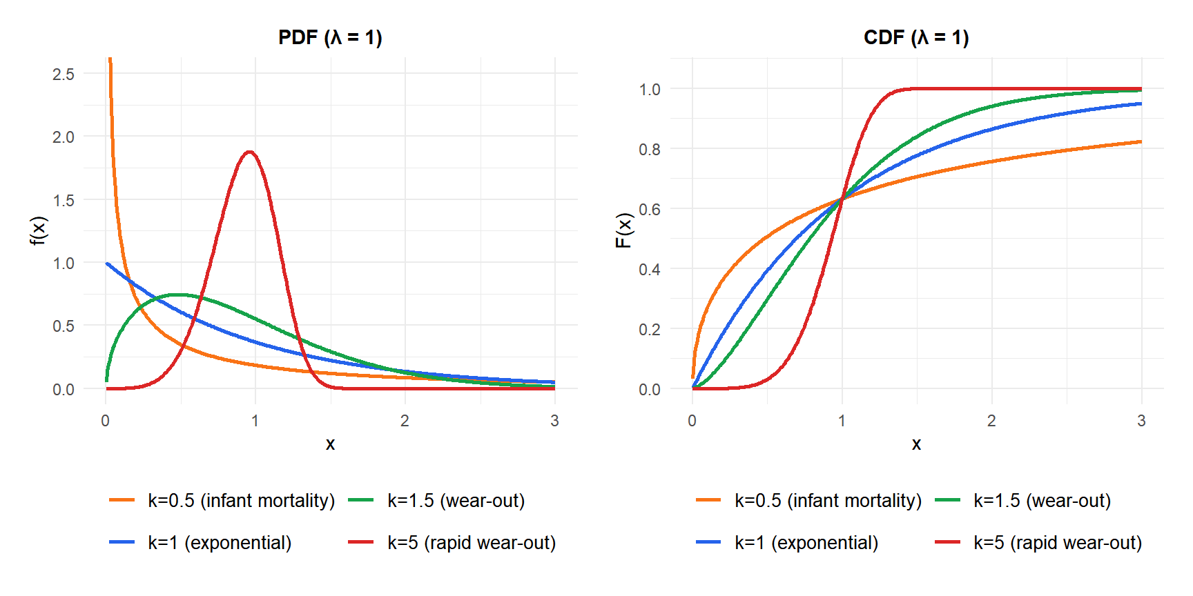
\[f(x) = \frac{k}{\lambda}\left(\frac{x}{\lambda}\right)^{k-1} e^{-(x/\lambda)^k}, \quad x \geq 0\]
The CDF has a clean closed form:
\[F(x) = 1 - e^{-(x/\lambda)^k}, \quad x \geq 0\]
⚠️ Parameter notation varies by source and software
Different sources use different symbols for the same parameters:
- R uses
shape(\(k\)) andscale(\(\lambda\)):dweibull(x, shape = k, scale = lambda). - Some engineering textbooks write the PDF as \(f(x) = \frac{\beta}{\eta}(x/\eta)^{\beta-1}e^{-(x/\eta)^\beta}\), where \(\beta = k\) (shape) and \(\eta = \lambda\) (characteristic life).
- Some sources use the rate \(\lambda' = 1/\lambda\) instead of the scale \(\lambda\).
Always check which convention your source uses before plugging numbers into a formula.
The shape parameter: three failure regimes
The shape parameter \(k\) determines how the failure rate evolves over time, which is the central question in reliability analysis:
- \(k < 1\): failure rate decreases over time. Failures are concentrated early in the component’s life (infant mortality, early defects). Items that survive the initial period become increasingly reliable.
- \(k = 1\): failure rate is constant. The Weibull reduces to the exponential distribution. Failures occur randomly, independent of age.
- \(k > 1\): failure rate increases over time. Components wear out and become more likely to fail as they age. Most mechanical components fall in this category.
Hazard function
The hazard function (also called failure rate or hazard rate) is the instantaneous rate of failure at time \(x\), given survival up to \(x\):
\[h(x) = \frac{f(x)}{1 - F(x)} = \frac{k}{\lambda}\left(\frac{x}{\lambda}\right)^{k-1}\]
For the Weibull, the hazard function is a power of \(x\):
- \(k < 1\): \(h(x)\) is decreasing (early failures dominate).
- \(k = 1\): \(h(x) = 1/\lambda\) is constant (memoryless, exponential).
- \(k > 1\): \(h(x)\) is increasing (aging, wear-out).
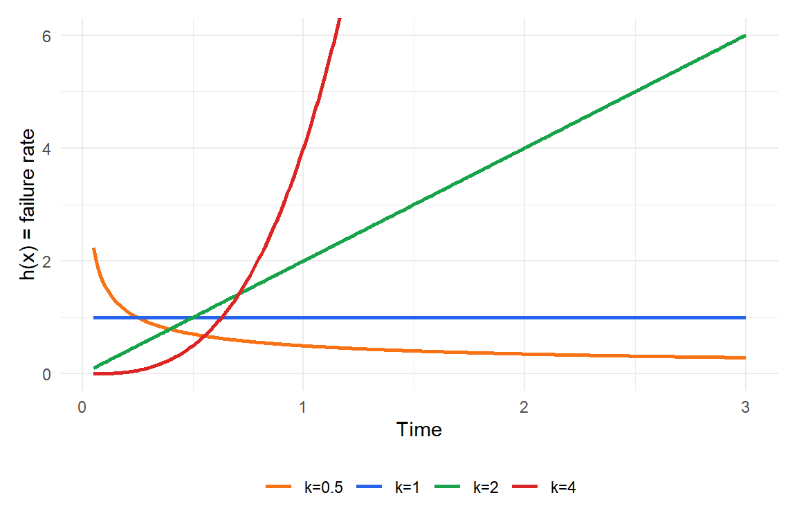
Figure 1: Hazard function: k<1 gives decreasing failure rate (infant mortality), k=1 constant (exponential), k>1 increasing (wear-out)
💡 The bathtub curve
In reliability engineering, the lifetime of a population of components often follows the “bathtub curve”: high early failure rate (infant mortality, \(k < 1\)), then a stable low rate during useful life (\(k \approx 1\)), then increasing rate as components age (\(k > 1\)). The Weibull distribution models each phase separately. In practice, the full bathtub curve requires a mixture of Weibull distributions with different shape parameters.
Properties
For \(X \sim \text{Weibull}(k, \lambda)\):
- Expected Value (Mean)
\[E(X) = \lambda\,\Gamma\!\left(1 + \frac{1}{k}\right)\]
where \(\Gamma\) is the gamma function. For \(k = 2\), \(\lambda = 5\): \(E(X) = 5\,\Gamma(1.5) = 5 \times 0.886 \approx 4.43\).
- Variance
\[\text{Var}(X) = \lambda^2\left[\Gamma\!\left(1 + \frac{2}{k}\right) - \left(\Gamma\!\left(1 + \frac{1}{k}\right)\right)^2\right]\]
- Skewness
\[\text{Skewness} = \frac{\Gamma(1 + 3/k)\lambda^3 - 3E(X)\text{Var}(X) - E(X)^3}{\text{Var}(X)^{3/2}}\]
Positive for \(k < 3.6\), approximately zero for \(k \approx 3.6\), slightly negative for larger \(k\).
- Median
\[\text{Median} = \lambda(\ln 2)^{1/k}\]
- Mode
\[\text{Mode} = \lambda\left(\frac{k-1}{k}\right)^{1/k}, \quad \text{for } k > 1\]
For \(k \leq 1\), the mode is 0.
- Quantile Function
\[Q(p) = \lambda\left(-\ln(1-p)\right)^{1/k}\]
Step-by-step example
A turbine blade has a lifetime following \(\text{Weibull}(k=2.5, \lambda=1000)\) hours.
Probability of failure within 500 hours:
\[F(500) = 1 - e^{-(500/1000)^{2.5}} = 1 - e^{-0.177} \approx 0.162\]
About 16.2% of blades fail within 500 hours.
Expected lifetime:
\[E(X) = 1000\,\Gamma(1 + 1/2.5) = 1000\,\Gamma(1.4) \approx 1000 \times 0.887 = 887 \text{ hours}\]
Median lifetime:
\[Q(0.5) = 1000(\ln 2)^{1/2.5} = 1000 \times 0.693^{0.4} \approx 1000 \times 0.860 = 860 \text{ hours}\]
90th percentile (design life that 90% of blades reach):
\[Q(0.90) = 1000(-\ln 0.10)^{1/2.5} = 1000 \times 2.303^{0.4} \approx 1000 \times 1.406 = 1{,}406 \text{ hours}\]
In a clinical trial, time-to-relapse follows \(\text{Weibull}(k=2, \lambda=5)\) years (\(k>1\) because relapse risk increases with time post-treatment).
- Median time to relapse: \(5(\ln 2)^{1/2} \approx 5 \times 0.833 = 4.16\) years.
- Probability of relapse-free survival past 3 years: \(P(X > 3) = e^{-(3/5)^2} = e^{-0.36} \approx 0.698\) (about 70%).
- Probability of relapse-free survival past 7 years: \(e^{-(7/5)^2} = e^{-1.96} \approx 0.141\) (about 14%).
💡 Relationship with other distributions
- Exponential: \(\text{Weibull}(1, \lambda) = \text{Exp}(1/\lambda)\). Constant hazard rate.
- Rayleigh: \(\text{Weibull}(2, \lambda)\). Used for wind speed modeling.
- Gamma: both generalize the exponential, but differently. The Gamma models the sum of exponential waiting times; the Weibull models a single waiting time with a non-constant rate.
- Extreme value: if \(X \sim \text{Weibull}(k, \lambda)\), then \(\ln(X)\) follows a Gumbel (extreme value) distribution.

