Student's t distribution
Student’s t distribution is what you use when you want to make inferences about a population mean but do not know the population variance. It is heavier-tailed than the normal and converges to it as sample size grows, making it the standard tool for t-tests and confidence intervals.
Definition
If \(Z \sim N(0,1)\) and \(V \sim \chi^2(\nu)\) are independent, then:
\[T = \frac{Z}{\sqrt{V/\nu}} \sim t(\nu)\]
\(T\) follows a Student’s t distribution with \(\nu\) degrees of freedom. Its PDF is:
\[f(x) = \frac{\Gamma\!\left(\frac{\nu+1}{2}\right)}{\sqrt{\nu\pi}\;\Gamma\!\left(\frac{\nu}{2}\right)} \left(1 + \frac{x^2}{\nu}\right)^{-(\nu+1)/2}, \quad -\infty < x < \infty\]
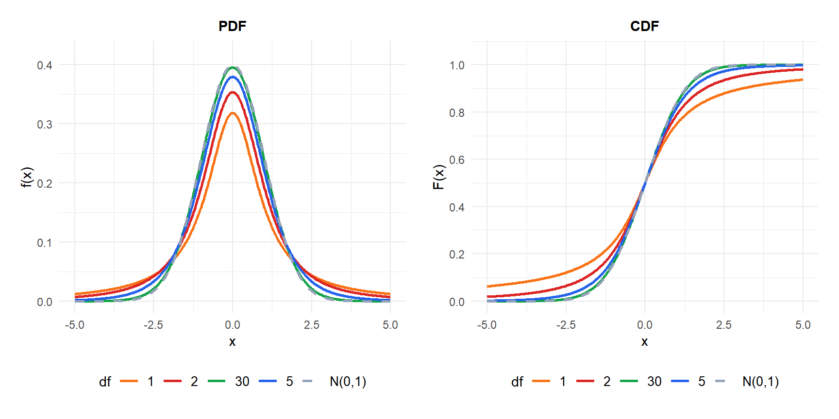
The distribution is symmetric around zero and bell-shaped like the normal, but with heavier tails. As \(\nu \to \infty\), \(t(\nu) \to N(0,1)\).
⚠️ Who is Student?
“Student” was the pseudonym of William Sealy Gosset, a statistician working at the Guinness brewery in Dublin in the early 1900s. Guinness did not allow employees to publish research, so Gosset published under the pen name “Student” in 1908. He developed the distribution to deal with small samples of barley and hops, making it one of the most practical origins of a fundamental statistical result.
Effect of degrees of freedom
The degrees of freedom \(\nu\) control how heavy the tails are:
- Small \(\nu\): very heavy tails. Extreme values are much more likely than under the normal. With \(\nu = 1\), the distribution is a Cauchy, which has no mean.
- \(\nu \geq 30\): practically indistinguishable from \(N(0,1)\) for most purposes.
- \(\nu \to \infty\): converges to \(N(0,1)\) exactly.
Properties
For \(T \sim t(\nu)\):
- Expected Value (Mean)
\[E(T) = 0, \quad \text{for } \nu > 1\]
Undefined for \(\nu = 1\) (Cauchy distribution).
- Variance
\[\text{Var}(T) = \frac{\nu}{\nu - 2}, \quad \text{for } \nu > 2\]
Undefined for \(\nu \leq 2\). Always greater than 1, approaching 1 as \(\nu \to \infty\).
- Skewness
Always 0: the distribution is perfectly symmetric around 0, for \(\nu > 3\).
- Kurtosis
\[g_2 = \frac{6}{\nu - 4}, \quad \text{for } \nu > 4\]
Always positive (leptokurtic). Approaches 0 as \(\nu \to \infty\).
- Mode and Median
Both equal 0 by symmetry.
- Quantile Function
No closed form; values are read from t-tables or computed with software. Key values for \(t_{0.975, \nu}\) (two-sided 95% CI):
| \(\nu\) | \(t_{0.975}\) |
|---|---|
| 5 | 2.571 |
| 10 | 2.228 |
| 20 | 2.086 |
| 30 | 2.042 |
| \(\infty\) | 1.960 |
As \(\nu\) grows, the critical value approaches 1.960, the standard normal quantile.
Why use t instead of z?
When testing a hypothesis about a population mean \(\mu\), the natural statistic is:
\[Z = \frac{\bar{X} - \mu}{\sigma / \sqrt{n}}\]
This follows \(N(0,1)\) exactly. The problem: \(\sigma\) is almost never known. Replacing it with the sample standard deviation \(S\) gives:
\[T = \frac{\bar{X} - \mu}{S / \sqrt{n}} \sim t(n-1)\]
This follows a t distribution because \(S\) introduces additional variability. The t distribution has heavier tails than the normal to account for the extra uncertainty from estimating \(\sigma\).
⚠️ When can you use z instead of t?
In practice, many textbooks say “use z when \(n \geq 30\) and \(\sigma\) is known, use t otherwise.” The real rule is simpler: always use t when \(\sigma\) is unknown, regardless of sample size. For large \(n\), \(t\) and \(z\) give nearly identical results anyway, so using \(t\) is never wrong.
The only case where \(z\) is strictly correct and \(t\) is an approximation is when \(\sigma\) is truly known, which is rare outside of controlled experiments.
Applications
One-sample t-test and confidence interval
To test \(H_0: \mu = \mu_0\) or construct a CI for \(\mu\):
\[T = \frac{\bar{X} - \mu_0}{S/\sqrt{n}} \sim t(n-1)\]
A \((1-\alpha)\) confidence interval for \(\mu\):
\[\bar{X} \pm t_{\alpha/2,\, n-1} \cdot \frac{S}{\sqrt{n}}\]
A food company claims its packages weigh 500 g on average. A quality auditor weighs 12 packages and finds \(\bar{X} = 494\) g and \(S = 8\) g.
Test \(H_0: \mu = 500\) vs \(H_1: \mu \neq 500\) at \(\alpha = 0.05\).
\[T = \frac{494 - 500}{8/\sqrt{12}} = \frac{-6}{2.309} \approx -2.60\]
Critical value: \(t_{0.025,\, 11} \approx 2.201\).
Since \(|{-2.60}| > 2.201\), we reject \(H_0\). There is significant evidence that the packages weigh less than claimed.
95% CI: \(494 \pm 2.201 \times 2.309 = 494 \pm 5.08 = (488.9,\ 499.1)\) g.
Two-sample t-test
To compare means of two independent groups with equal variances:
\[T = \frac{\bar{X}_1 - \bar{X}_2}{S_p\sqrt{1/n_1 + 1/n_2}} \sim t(n_1 + n_2 - 2)\]
where \(S_p^2 = \frac{(n_1-1)S_1^2 + (n_2-1)S_2^2}{n_1+n_2-2}\) is the pooled variance.
For unequal variances, Welch’s t-test uses a modified degrees of freedom (Satterthwaite approximation).
⚠️ Always check the equal variance assumption
The pooled two-sample t-test assumes equal variances. If variances differ substantially, use Welch’s t-test instead: it does not assume equal variances and is generally recommended as the default. In R, t.test() uses Welch by default; add var.equal = TRUE for the pooled version.
Paired t-test
When observations come in pairs (before/after, matched subjects), compute the differences \(D_i = X_{i1} - X_{i2}\) and apply a one-sample t-test to \(D_i\).
Eight employees complete a typing speed test before and after a training program. The differences (after minus before, in words per minute) are:
\[d = (5, 8, -2, 12, 6, 3, 9, 4)\]
\(\bar{d} = 5.625\), \(S_d \approx 4.24\), \(n = 8\).
\[T = \frac{5.625}{4.24/\sqrt{8}} = \frac{5.625}{1.499} \approx 3.75\]
Critical value: \(t_{0.025,\, 7} \approx 2.365\).
Since \(3.75 > 2.365\), we reject \(H_0\): training significantly improved typing speed (\(p \approx 0.007\)).
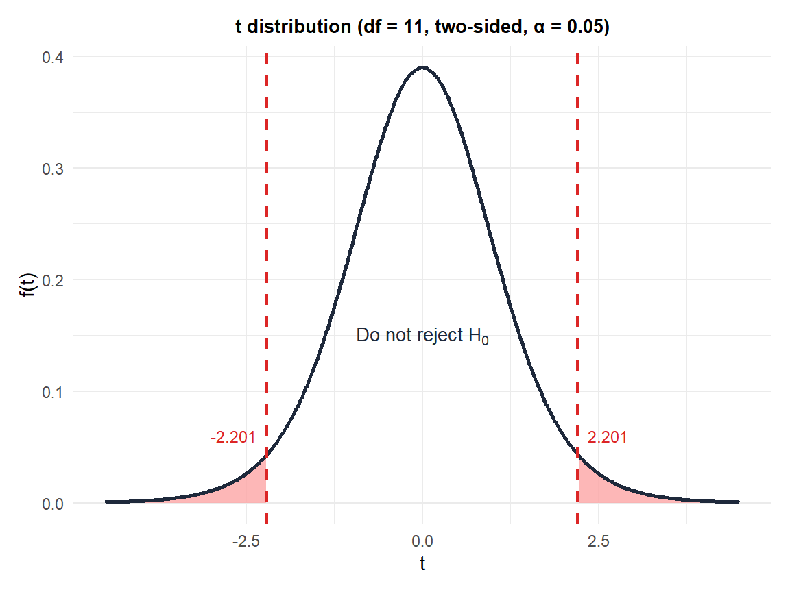
Figure 1: Two-sided t-test with 11 degrees of freedom at α=0.05: rejection regions in red
💡 Relationship with other distributions
- Normal: \(t(\infty) = N(0,1)\). As \(\nu \to \infty\), the t converges to the standard normal.
- Cauchy: \(t(1) = \text{Cauchy}(0,1)\). No mean, no variance.
- Chi-squared: \(T^2 \sim F(1, \nu)\) where \(F\) is the F distribution. Squaring a t statistic gives an F statistic.
- F distribution: \(t(\nu)^2 = F(1, \nu)\).
- Beta: \(T^2/(\nu + T^2) \sim \text{Beta}(1/2, \nu/2)\).

