Normal distribution
The normal distribution is the most important continuous distribution in statistics. It describes an enormous variety of natural phenomena, and it is the limiting distribution of sums and averages of independent random variables, which is why it appears everywhere.
Definition
A random variable \(X\) follows a normal distribution with mean \(\mu \in \mathbb{R}\) and standard deviation \(\sigma > 0\), written \(X \sim N(\mu, \sigma)\), if its probability density function is:
\[f(x) = \frac{1}{\sigma\sqrt{2\pi}}\, e^{-\frac{(x-\mu)^2}{2\sigma^2}}, \quad -\infty < x < \infty\]
The curve is bell-shaped, symmetric around \(\mu\), and its spread is controlled by \(\sigma\). The total area under the curve is always 1.
⚠️ Notation: N(μ, σ) vs N(μ, σ²)
Different textbooks use different conventions:
- \(N(\mu, \sigma)\): parametrized by mean and standard deviation. Common in many European and Spanish-language textbooks.
- \(N(\mu, \sigma^2)\): parametrized by mean and variance. Common in Anglo-Saxon statistics textbooks and most software documentation.
Always check which convention your course uses before plugging numbers into formulas. A normal distribution with mean 0 and standard deviation 2 is \(N(0, 2)\) in one convention and \(N(0, 4)\) in the other.
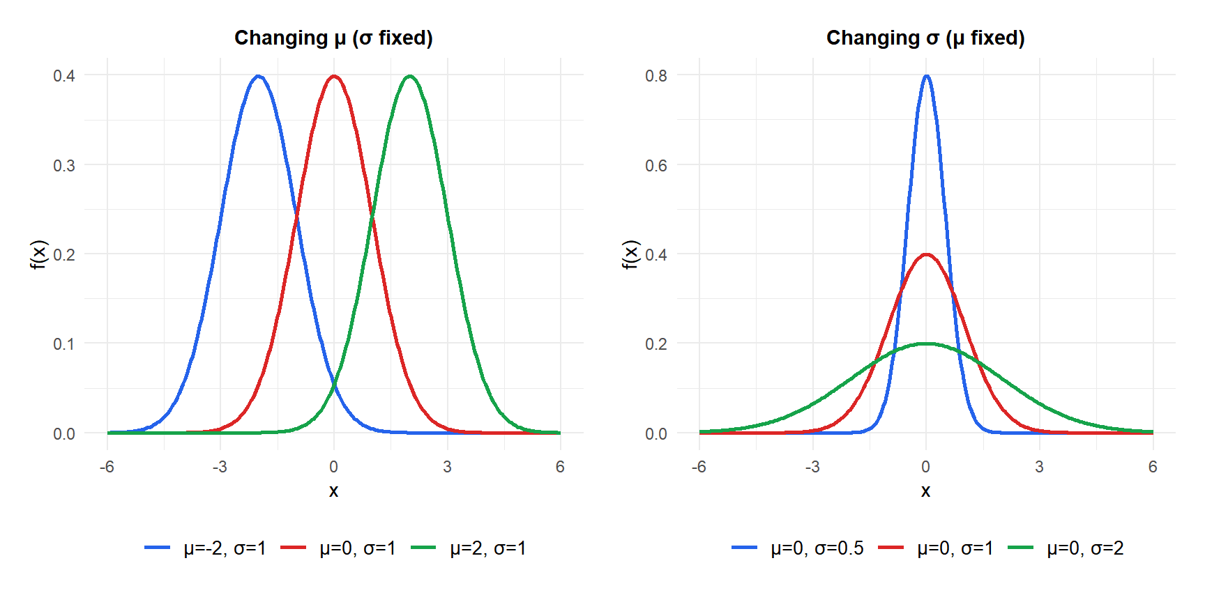
Figure 1: Effect of changing μ (left) and σ (right) on the normal distribution shape
Properties
For \(X \sim N(\mu, \sigma)\):
- Expected Value (Mean)
\[E(X) = \mu\]
- Variance
\[\text{Var}(X) = \sigma^2\]
- Skewness
Always 0. The normal distribution is perfectly symmetric around \(\mu\).
- Kurtosis
\[g_2 = 0 \quad \text{(excess kurtosis)}\]
The normal distribution is the reference for kurtosis: mesokurtic by definition. Raw kurtosis is 3; excess kurtosis subtracts 3 to give 0.
- Mode and Median
\[\text{Mode} = \text{Median} = \mu\]
All three measures of central tendency coincide, a consequence of perfect symmetry.
- CDF
\[F(x) = \Phi\left(\frac{x-\mu}{\sigma}\right) = \frac{1}{2}\left[1 + \text{erf}\left(\frac{x-\mu}{\sigma\sqrt{2}}\right)\right]\]
where \(\Phi\) is the standard normal CDF. There is no closed-form antiderivative: probabilities are computed numerically or from tables.
- Quantile Function
\[Q(p) = \mu + \sigma\,\Phi^{-1}(p)\]
The 95th percentile of \(N(0,1)\) is \(\Phi^{-1}(0.95) \approx 1.645\).
The 68-95-99.7 rule
The most practical result about the normal distribution is the empirical rule: almost all of the probability is concentrated within a few standard deviations of the mean.
\[P(\mu - \sigma \leq X \leq \mu + \sigma) \approx 0.6827\] \[P(\mu - 2\sigma \leq X \leq \mu + 2\sigma) \approx 0.9545\] \[P(\mu - 3\sigma \leq X \leq \mu + 3\sigma) \approx 0.9973\]
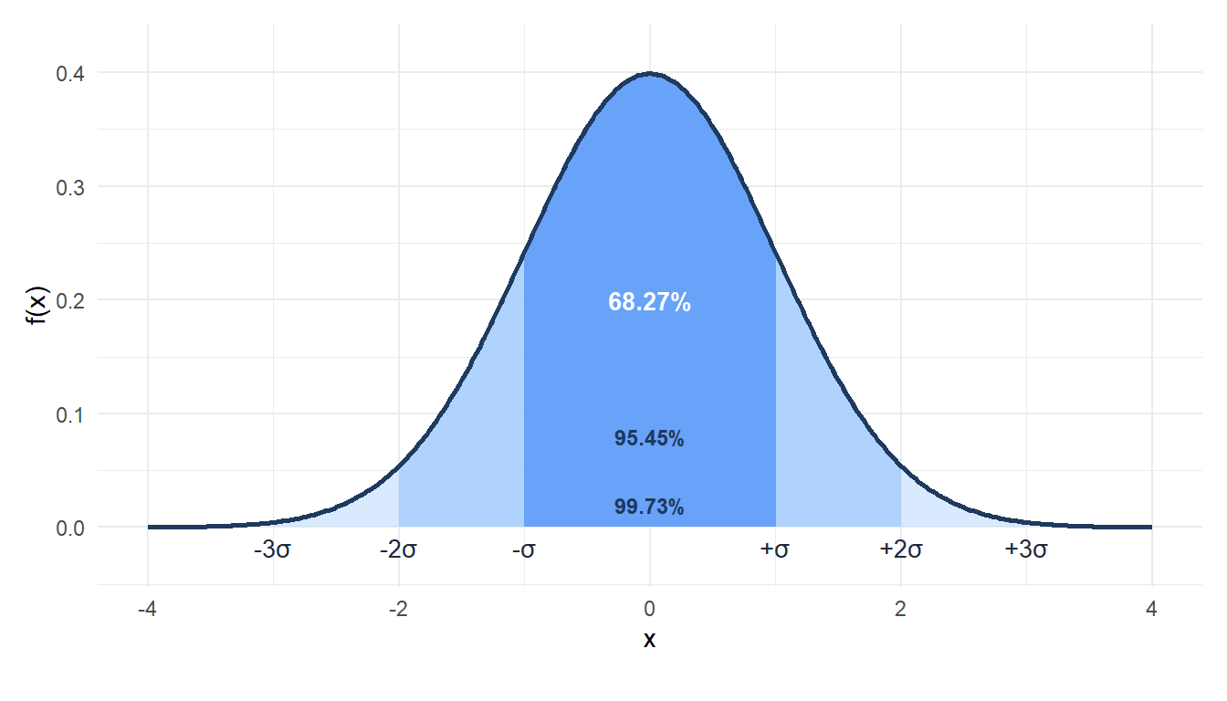
Figure 2: The 68-95-99.7 rule: probability within 1, 2 and 3 standard deviations of the mean
Adult male height in a country follows \(N(175, 7)\) cm (mean 175 cm, SD 7 cm).
- About 68% of men are between \(175 - 7 = 168\) and \(175 + 7 = 182\) cm.
- About 95% are between \(175 - 14 = 161\) and \(175 + 14 = 189\) cm.
- Only about 0.3% are below 154 cm or above 196 cm (more than 3 SDs from the mean).
Standard normal distribution
The standard normal distribution \(Z \sim N(0, 1)\) has mean 0 and standard deviation 1. Its PDF is:
\[f(z) = \frac{1}{\sqrt{2\pi}}\,e^{-z^2/2}, \quad -\infty < z < \infty\]
Its CDF is denoted \(\Phi(z) = P(Z \leq z)\) and is tabulated in standard normal tables.
Any normal variable can be standardized:
\[Z = \frac{X - \mu}{\sigma}\]
This converts \(X \sim N(\mu, \sigma)\) to \(Z \sim N(0,1)\), allowing the use of a single table for all normal distributions.
Useful symmetry properties of \(\Phi\): - \(\Phi(-z) = 1 - \Phi(z)\) - \(P(Z > z) = 1 - \Phi(z)\) - \(P(a \leq Z \leq b) = \Phi(b) - \Phi(a)\)
Step-by-step example
The scores on a standardized exam follow \(X \sim N(70, 10)\) (mean 70, SD 10).
Probability of scoring above 85:
Standardize: \(z = (85 - 70)/10 = 1.5\)
\[P(X > 85) = P(Z > 1.5) = 1 - \Phi(1.5) \approx 1 - 0.9332 = 0.0668\]
About 6.7% of students score above 85.
Probability of scoring between 60 and 80:
\[P(60 \leq X \leq 80) = \Phi\left(\frac{80-70}{10}\right) - \Phi\left(\frac{60-70}{10}\right) = \Phi(1) - \Phi(-1) \approx 0.8413 - 0.1587 = 0.6827\]
This is exactly the 68.27% from the empirical rule: the interval \([\mu - \sigma, \mu + \sigma]\).
Score at the 90th percentile:
\[Q(0.90) = 70 + 10 \times \Phi^{-1}(0.90) \approx 70 + 10 \times 1.282 = 82.82\]
A student needs to score about 82.8 to be in the top 10%.
Why the normal distribution is everywhere
The Central Limit Theorem (CLT) states that the sum (or average) of a large number of independent random variables, regardless of their individual distributions, tends toward a normal distribution. This is the mathematical reason why the normal distribution appears in so many natural and social phenomena:
- Heights and weights result from many small genetic and environmental factors summing up.
- Measurement errors in physics are sums of many small independent sources of error.
- Sample means in statistical inference are approximately normal for large samples, regardless of the population distribution.
💡 Relationship with other distributions
- Standard normal: \(N(0, 1)\) is the reference. All other normal distributions are shifts and scalings of it.
- Chi-squared: the sum of squares of \(k\) independent \(N(0,1)\) variables follows \(\chi^2(k)\).
- Student’s t: the ratio of a \(N(0,1)\) variable to the square root of a \(\chi^2(k)/k\) variable.
- Log-normal: if \(\ln(X) \sim N(\mu, \sigma)\), then \(X\) follows a log-normal distribution. Used for asset prices and biological measurements that cannot be negative.
- Binomial approximation: \(\text{Binomial}(n,p) \approx N(np, \sqrt{np(1-p)})\) for large \(n\).

