Negative binomial distribution
The negative binomial distribution models the number of failures before a target number of successes in a sequence of independent Bernoulli trials. It is also widely used as a flexible model for overdispersed count data, where the variance exceeds the mean.
Definition
A random variable \(X\) follows a negative binomial distribution with parameters \(r > 0\) (number of successes) and \(p \in (0,1)\) (probability of success per trial), written \(X \sim \text{NegBin}(r, p)\), if:
\[P(X = k) = \binom{k + r - 1}{k} p^r (1-p)^k, \quad k = 0, 1, 2, \ldots\]
where \(k\) is the number of failures before the \(r\)-th success.
The negative binomial generalizes the geometric distribution: when \(r = 1\), it reduces to the number of failures before the first success.
⚠️ Two parametrizations - know which one your software uses
The negative binomial has two common parametrizations:
1. Counting failures (used above): \(X\) = number of failures before \(r\) successes. Parameters: \(r\) (successes) and \(p\) (success probability). This is the textbook version.
2. Overdispersion model (used in R, Python, most regression software): \(X\) = count of events, parametrized by mean \(\mu\) and dispersion parameter \(r\) (also called size). The PMF is:
\[P(X = k) = \binom{k + r - 1}{k} \left(\frac{r}{r + \mu}\right)^r \left(\frac{\mu}{r + \mu}\right)^k\]
with \(\text{Var}(X) = \mu + \mu^2/r > \mu\). As \(r \to \infty\), variance approaches mean and the distribution converges to Poisson.
In R: dnbinom(x, size = r, prob = p) uses parametrization 1; dnbinom(x, size = r, mu = mu) uses parametrization 2.
Probability Mass Function and CDF
The CDF accumulates the PMF:
\[F(k) = P(X \leq k) = \sum_{i=0}^{k} \binom{i+r-1}{i} p^r (1-p)^i\]
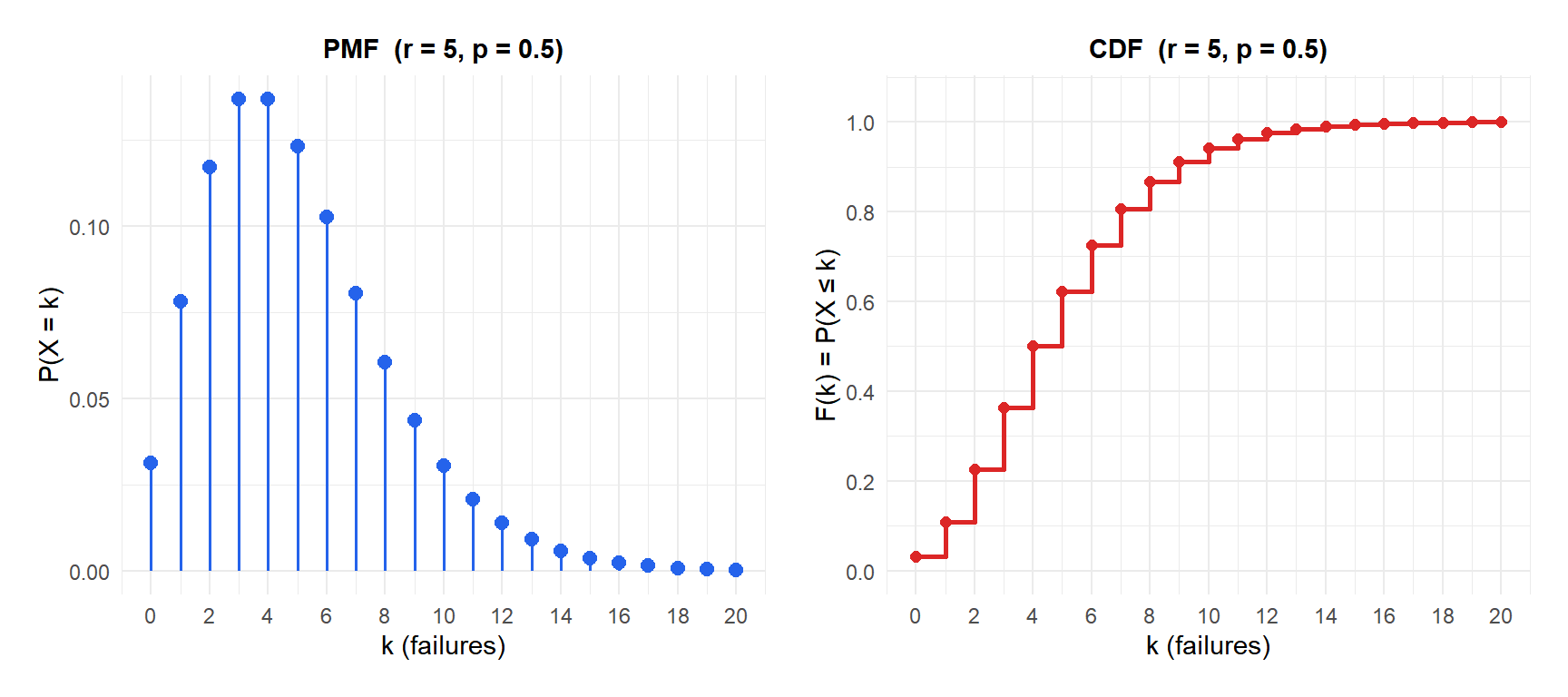
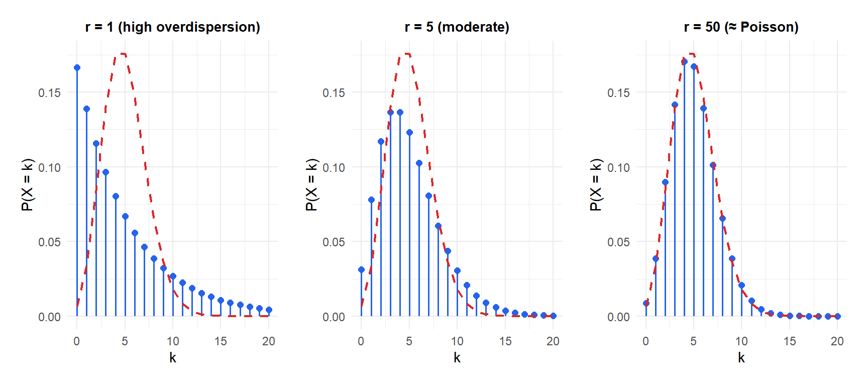
Figure 1: As the dispersion parameter r increases, the negative binomial converges to Poisson (same mean, less overdispersion)
Properties
For \(X \sim \text{NegBin}(r, p)\) in the failures-before-successes parametrization:
- Expected Value (Mean)
\[E(X) = \frac{r(1-p)}{p}\]
- Variance
\[\text{Var}(X) = \frac{r(1-p)}{p^2}\]
Since \(\text{Var}(X) = E(X)/p > E(X)\) for \(p < 1\), the negative binomial always has variance greater than its mean: this is overdispersion by construction.
- Skewness
\[\text{Skewness} = \frac{2 - p}{\sqrt{r(1-p)}}\]
- Kurtosis
\[g_2 = \frac{6}{r} + \frac{p^2}{r(1-p)}\]
- Mode
\[\text{Mode} = \left\lfloor \frac{(r-1)(1-p)}{p} \right\rfloor \quad \text{for } r > 1\]
When \(r = 1\) (geometric), the mode is 0.
- Quantile Function
No closed form; computed numerically.
Step-by-step example
A pharmaceutical sales representative needs to close 3 deals (\(r = 3\)). Each sales call succeeds with probability \(p = 0.2\). Let \(X\) = number of failed calls before the 3rd success, \(X \sim \text{NegBin}(3, 0.2)\).
Probability of exactly 7 failures before the 3rd success:
\[P(X = 7) = \binom{7+3-1}{7}(0.2)^3(0.8)^7 = \binom{9}{7}(0.008)(0.2097) \approx 36 \times 0.001678 \approx 0.0604\]
Expected number of failed calls:
\[E(X) = \frac{3 \times 0.8}{0.2} = 12 \text{ failures}\]
Variance:
\[\text{Var}(X) = \frac{3 \times 0.8}{0.04} = 60\]
The standard deviation is \(\sqrt{60} \approx 7.75\), reflecting the wide spread: some reps will close quickly, others will need many more calls.
A health researcher counts the number of doctor visits per year for 500 patients. The sample mean is 3.2 visits and the sample variance is 8.7. Since variance (8.7) is much larger than the mean (3.2), a Poisson model is inadequate.
Fitting a negative binomial with \(\mu = 3.2\) and estimated \(r = 2.1\):
\[\text{Var}(X) = \mu + \frac{\mu^2}{r} = 3.2 + \frac{10.24}{2.1} \approx 3.2 + 4.9 = 8.1\]
The negative binomial captures the overdispersion that the Poisson cannot.
Overdispersion and the Poisson connection
The negative binomial is the standard alternative to the Poisson when count data shows overdispersion. As \(r \to \infty\) with \(\mu = r(1-p)/p\) fixed, the negative binomial converges to \(\text{Poisson}(\mu)\). The parameter \(r\) controls how much extra variance there is beyond the Poisson: small \(r\) means heavy overdispersion, large \(r\) means close to Poisson.
In practice, a negative binomial regression model is fitted whenever a Poisson regression shows signs of overdispersion (residual deviance much larger than degrees of freedom, or a dispersion test is significant).
💡 Relationship with other distributions
- Geometric: NegBin\((1, p)\) = Geometric\((p)\) (failures before first success).
- Poisson: limiting case as \(r \to \infty\) with mean fixed.
- Binomial: NegBin counts failures in an unlimited sequence; Binomial counts successes in a fixed number of trials.
- Gamma-Poisson mixture: the negative binomial arises naturally when \(\lambda\) in a Poisson model follows a Gamma distribution, explaining why it handles heterogeneity in the population.

