Lognormal distribution
The lognormal distribution models variables that are always positive and right-skewed, where the logarithm of the variable follows a normal distribution. It appears naturally whenever a quantity is the product of many independent random factors.
Definition
A random variable \(X\) follows a lognormal distribution with parameters \(\mu \in \mathbb{R}\) and \(\sigma > 0\), written \(X \sim \text{Lognormal}(\mu, \sigma)\), if \(Y = \ln(X) \sim N(\mu, \sigma)\).
Its probability density function is:
\[f(x) = \frac{1}{x\sigma\sqrt{2\pi}}\exp\left(-\frac{(\ln x - \mu)^2}{2\sigma^2}\right), \quad x > 0\]
⚠️ μ and σ are parameters of ln(X), not of X itself
This is the most common source of confusion. In \(X \sim \text{Lognormal}(\mu, \sigma)\):
- \(\mu\) is the mean of \(\ln(X)\), not of \(X\).
- \(\sigma\) is the standard deviation of \(\ln(X)\), not of \(X\).
The actual mean of \(X\) is \(e^{\mu + \sigma^2/2}\), which is always larger than \(e^\mu\). If someone tells you “this variable has a lognormal distribution with mean 0 and SD 1”, they almost certainly mean that \(\ln(X) \sim N(0,1)\), not that \(E(X) = 0\).
The CDF has a clean form in terms of the standard normal CDF \(\Phi\):
\[F(x) = \Phi\left(\frac{\ln x - \mu}{\sigma}\right)\]
This makes probability calculations straightforward: standardize \(\ln(x)\) and look up the standard normal table.
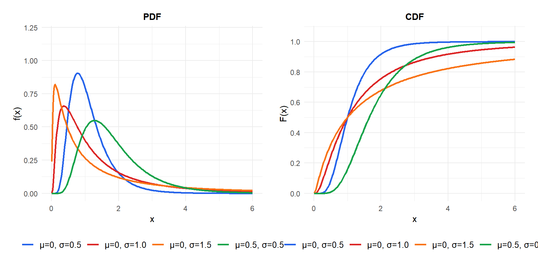
PDF and CDF
Properties
For \(X \sim \text{Lognormal}(\mu, \sigma)\):
- Expected Value (Mean)
\[E(X) = e^{\mu + \sigma^2/2}\]
- Variance
\[\text{Var}(X) = \left(e^{\sigma^2} - 1\right)e^{2\mu + \sigma^2}\]
- Median
\[\text{Median}(X) = e^{\mu}\]
The median is always less than the mean (since \(e^{\mu} < e^{\mu + \sigma^2/2}\)), reflecting the right skew.
- Mode
\[\text{Mode}(X) = e^{\mu - \sigma^2}\]
The mode is the smallest of the three: Mode \(<\) Median \(<\) Mean, a hallmark of right-skewed distributions.
- Skewness
\[\text{Skewness} = \left(e^{\sigma^2} + 2\right)\sqrt{e^{\sigma^2} - 1}\]
Always positive. For \(\sigma = 1\): skewness \(\approx 6.18\).
- Kurtosis
\[g_2 = e^{4\sigma^2} + 2e^{3\sigma^2} + 3e^{2\sigma^2} - 6\]
For \(\sigma = 1\): \(g_2 \approx 110.9\), extremely leptokurtic. The lognormal has very heavy tails for large \(\sigma\).
- Quantile Function
\[Q(p) = e^{\mu + \sigma\,\Phi^{-1}(p)}\]
where \(\Phi^{-1}\) is the standard normal quantile function.
Why the lognormal appears in practice
The lognormal arises naturally whenever a quantity is the product of many independent positive random factors. By the Central Limit Theorem applied to logarithms:
\[\ln(X) = \ln(X_1 \cdot X_2 \cdots X_n) = \sum_{i=1}^n \ln(X_i) \xrightarrow{} N(\mu, \sigma)\]
So \(X\) is lognormal. This is why it describes:
- Stock prices: today’s price is yesterday’s price multiplied by a random return factor.
- Income distributions: salaries result from multiplicative adjustments over a career.
- Biological sizes: cell growth is multiplicative at each division.
- Repair times: each step in a repair process multiplies the previous duration.
💡 Log-transform and work in normal scale
The key practical advantage of the lognormal: if \(X\) is lognormal, then \(\ln(X)\) is normal, and all normal distribution tools apply. To find \(P(X \leq x)\), compute \(P(\ln X \leq \ln x) = \Phi((\ln x - \mu)/\sigma)\). To find the 90th percentile of \(X\), find the 90th percentile of \(\ln(X)\) and exponentiate. Working in log scale turns a lognormal problem into a normal problem.
Step-by-step example
The daily returns of a stock are approximately normal, so its price follows a lognormal process. Suppose the log-price changes have \(\mu = 0.001\) (daily drift) and \(\sigma = 0.02\) (daily volatility). The stock currently trades at 100 USD.
After one trading day, the price \(P \sim 100 \cdot \text{Lognormal}(0.001, 0.02)\).
Expected price tomorrow:
\[E(P) = 100 \cdot e^{0.001 + 0.02^2/2} = 100 \cdot e^{0.0012} \approx 100.12 \text{ USD}\]
Probability the price drops below 98 USD:
Standardize: \(z = (\ln(98/100) - 0.001)/0.02 = (\ln(0.98) - 0.001)/0.02 \approx (-0.0202 - 0.001)/0.02 \approx -1.06\)
\[P(P < 98) = \Phi(-1.06) \approx 0.145\]
About 14.5% chance of a drop below 98 USD in one day.
90th percentile of tomorrow’s price:
\[Q(0.90) = 100 \cdot e^{0.001 + 0.02 \times 1.282} \approx 100 \cdot e^{0.02664} \approx 102.70 \text{ USD}\]
Income: household incomes in a country follow approximately \(\text{Lognormal}(10.5, 0.8)\) (in local currency units). Mean income: \(e^{10.5 + 0.32} \approx e^{10.82} \approx 50{,}000\). Median income: \(e^{10.5} \approx 36{,}000\). The mean is 39% higher than the median, reflecting the long right tail of high earners.
Website response time: request latency often follows a lognormal distribution. If \(\mu = 2\) and \(\sigma = 0.5\) (in log-milliseconds), the median latency is \(e^2 \approx 7.4\) ms and the 99th percentile is \(e^{2 + 0.5 \times 2.326} \approx e^{3.163} \approx 23.6\) ms.
💡 Relationship with other distributions
- Normal: \(\ln(X) \sim N(\mu, \sigma)\) by definition.
- Exponential: a special case of lognormal is not exact, but both model positive right-skewed data. Use exponential for memoryless processes, lognormal for multiplicative ones.
- Pareto: for very heavy tails (power-law behavior), the Pareto distribution is more appropriate than the lognormal.
- Log-transformation in regression: log-linear regression models assume the response is lognormal given the predictors.

