Hypergeometric distribution
The hypergeometric distribution models the number of successes when drawing a sample without replacement from a finite population. Unlike the binomial, it accounts for the fact that each draw changes the composition of the remaining population.
Definition
A random variable \(X\) follows a hypergeometric distribution if it counts the number of successes in a sample of size \(n\) drawn without replacement from a population of size \(N\) containing \(K\) successes. Written \(X \sim \text{Hypergeometric}(N, K, n)\):
\[P(X = k) = \frac{\binom{K}{k}\binom{N-K}{n-k}}{\binom{N}{n}}, \quad \max(0,\, n-(N-K)) \leq k \leq \min(K, n)\]
The numerator counts the ways to choose \(k\) successes from the \(K\) available and \(n-k\) failures from the \(N-K\) available. The denominator counts all ways to choose \(n\) items from \(N\).
⚠️ Hypergeometric vs binomial: the key distinction
Both distributions count successes in a sample, but:
- Binomial: sampling with replacement. Each draw is independent and \(p\) stays constant.
- Hypergeometric: sampling without replacement. Each draw changes the population, so draws are dependent and \(p\) shifts after each one.
Use the hypergeometric when the sample is a meaningful fraction of the population (roughly \(n/N > 0.05\)). When the population is large relative to the sample, the two distributions give nearly identical results and the binomial is simpler to work with.
Probability Mass Function and CDF
The CDF sums the PMF up to \(k\):
\[F(k) = P(X \leq k) = \sum_{i=0}^{k} \frac{\binom{K}{i}\binom{N-K}{n-i}}{\binom{N}{n}}\]
Properties
For \(X \sim \text{Hypergeometric}(N, K, n)\), let \(p = K/N\) be the proportion of successes in the population:
- Expected Value (Mean)
\[E(X) = n\frac{K}{N} = np\]
The expected number of successes is the same as in the binomial with the same \(n\) and \(p = K/N\).
- Variance
\[\text{Var}(X) = n\frac{K}{N}\left(1 - \frac{K}{N}\right)\frac{N-n}{N-1} = np(1-p)\frac{N-n}{N-1}\]
The factor \(\frac{N-n}{N-1}\) is the finite population correction (FPC). It is always less than 1, making the hypergeometric variance smaller than the binomial variance \(np(1-p)\). This makes intuitive sense: sampling without replacement reduces uncertainty because you cannot get the same item twice.
- Skewness
\[\text{Skewness} = \frac{(N-2K)(N-2n)\sqrt{N-1}}{(N-2)\sqrt{nK(N-K)(N-n)}}\]
- Kurtosis
\[g_2 = \frac{(N-1)N^2[N(N+1) - 6K(N-K) - 6n(N-n)] + 6nK(N-K)(N-n)(5N-6)}{n K(N-K)(N-n)(N-2)(N-3)}\]
In practice, kurtosis is computed numerically for specific parameter values.
- Mode
\[\text{Mode} = \left\lfloor \frac{(n+1)(K+1)}{N+2} \right\rfloor\]
- Quantile Function
No closed form; computed numerically.
The finite population correction
The FPC factor \(\frac{N-n}{N-1}\) captures the effect of the finite population on variance:
- When \(n = 1\): FPC \(\approx 1\), variance equals the binomial variance.
- When \(n = N\) (census): FPC \(= 0\), variance equals zero. You have measured the entire population, so there is no sampling uncertainty.
- When \(n/N\) is small (say below 5%): FPC \(\approx 1\) and the hypergeometric is well approximated by the binomial.
A company has 200 employees, 60 of whom are managers (\(K = 60\), \(N = 200\)). A survey samples 40 employees (\(n = 40\)).
Binomial variance (ignoring finite population): \[np(1-p) = 40 \times 0.3 \times 0.7 = 8.4\]
Hypergeometric variance (with FPC): \[8.4 \times \frac{200-40}{200-1} = 8.4 \times \frac{160}{199} \approx 6.75\]
The actual variance is 20% smaller than the binomial would suggest. When \(n/N = 40/200 = 20\%\), the correction is substantial.
Step-by-step example
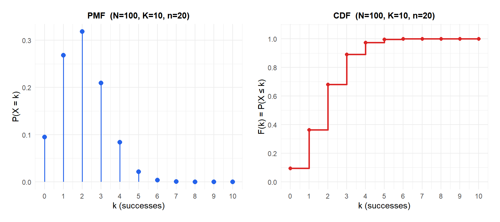
A factory batch contains 100 items, 10 of which are defective (\(N=100\), \(K=10\)). A quality inspector draws 20 items without replacement (\(n=20\)). Let \(X\) = number of defective items found.
Probability of exactly 3 defective items:
\[P(X=3) = \frac{\binom{10}{3}\binom{90}{17}}{\binom{100}{20}} \approx 0.141\]
There is a 14.1% chance of finding exactly 3 defective items.
Expected number of defectives:
\[E(X) = 20 \times \frac{10}{100} = 2\]
Variance:
\[\text{Var}(X) = 20 \times 0.1 \times 0.9 \times \frac{80}{99} \approx 1.455\]
Probability of finding at most 3 defectives:
\[F(3) = P(X=0) + P(X=1) + P(X=2) + P(X=3) \approx 0.069 + 0.271 + 0.385 + 0.141 = 0.866\]
About 87% of samples of size 20 will contain 3 or fewer defective items.
A standard deck has 52 cards, 4 of which are aces (\(N=52\), \(K=4\)). Five cards are dealt (\(n=5\)).
Probability of exactly 2 aces:
\[P(X=2) = \frac{\binom{4}{2}\binom{48}{3}}{\binom{52}{5}} = \frac{6 \times 17{,}296}{2{,}598{,}960} \approx 0.0399\]
Expected number of aces: \(E(X) = 5 \times 4/52 \approx 0.385\).
💡 When to use hypergeometric vs binomial
Use the hypergeometric when:
- Sampling is without replacement from a finite population.
- The sample is a substantial fraction of the population (\(n/N > 0.05\)).
Use the binomial instead when:
- Sampling is with replacement.
- The population is large enough that \(n/N \leq 0.05\): in this case the FPC \(\approx 1\) and the binomial gives nearly identical results with simpler calculations.
A common practical guideline: if you are sampling fewer than 5% of the population, the binomial approximation is adequate.

