Gamma distribution

The gamma distribution is a flexible continuous distribution that generalizes the exponential. While the exponential models the waiting time until the first event, the gamma models the waiting time until the \(k\)-th event in a Poisson process.

Definition

A random variable \(X\) follows a gamma distribution with shape parameter \(k > 0\) and rate parameter \(\lambda > 0\), written \(X \sim \text{Gamma}(k, \lambda)\), if its PDF is:

where \(\Gamma(k) = \int_0^\infty t^{k-1} e^{-t}\, dt\) is the gamma function. For positive integers, \(\Gamma(k) = (k-1)!\). For example, \(\Gamma(3) = 2! = 2\) and \(\Gamma(5) = 4! = 24\).

An equivalent parametrization uses the scale parameter \(\theta = 1/\lambda\):

\[f(x) = \frac{x^{k-1} e^{-x/\theta}}{\Gamma(k)\, \theta^k}, \quad x > 0\]

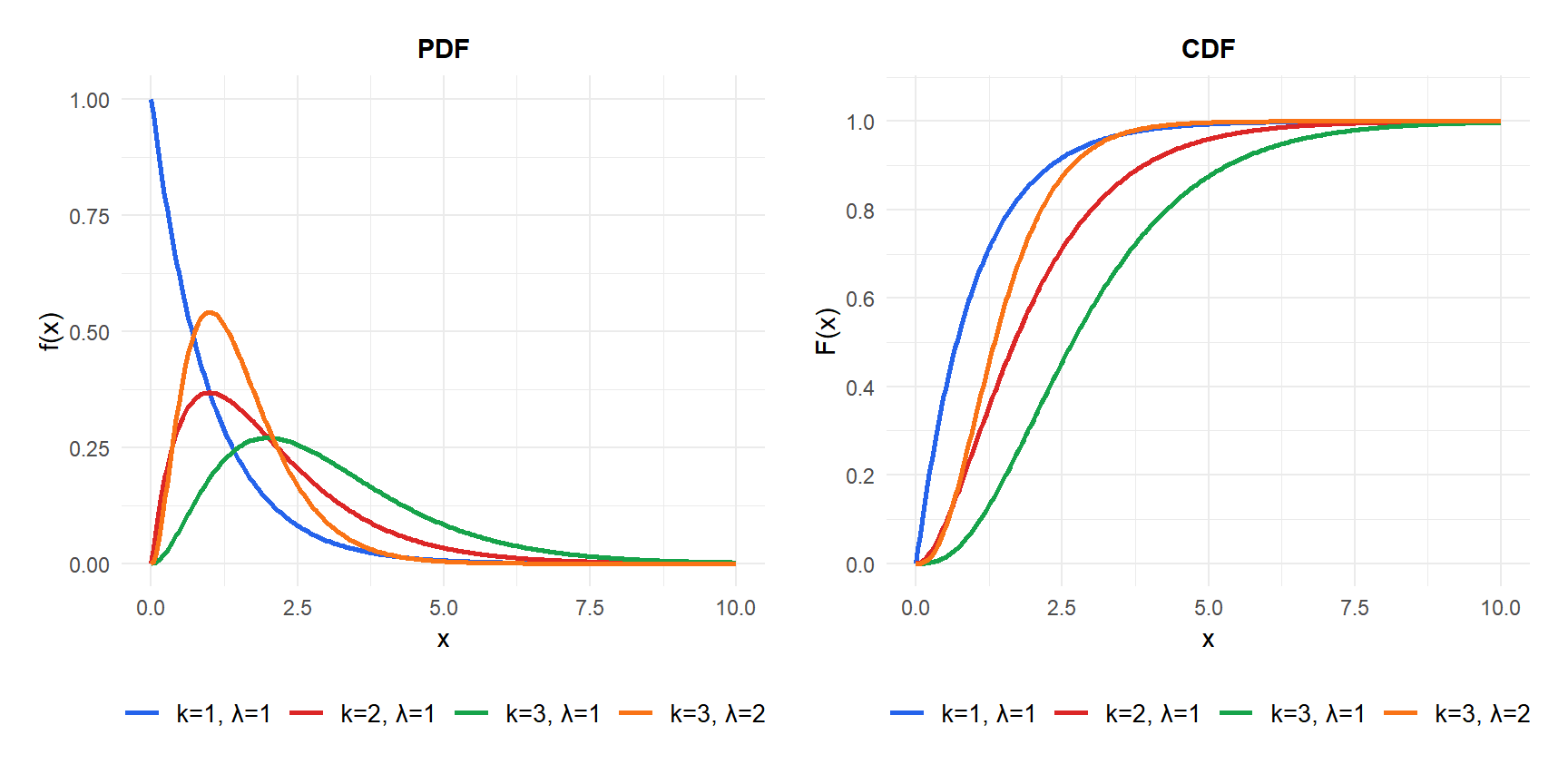
Probability Density Function and CDF

The CDF is expressed via the lower incomplete gamma function:

\[F(x) = \frac{\gamma(k,\, \lambda x)}{\Gamma(k)}\]

where \(\gamma(k, u) = \int_0^u t^{k-1} e^{-t}\, dt\). There is no closed form for general \(k\); probabilities are computed numerically.

Properties

For \(X \sim \text{Gamma}(k, \lambda)\):

1. Expected Value (Mean)

\[E(X) = \frac{k}{\lambda}\]

2. Variance

\[\text{Var}(X) = \frac{k}{\lambda^2}\]

3. Skewness

\[\text{Skewness} = \frac{2}{\sqrt{k}}\]

The distribution is right-skewed for small \(k\) and becomes increasingly symmetric as \(k\) grows. For large \(k\), the gamma approaches a normal distribution.

4. Kurtosis

\[g_2 = \frac{6}{k}\]

5. Mode

\[\text{Mode} = \frac{k-1}{\lambda} \quad \text{for } k \geq 1\]

For \(k < 1\), the distribution is monotonically decreasing and the mode is 0.

6. Quantile Function

No closed form; computed numerically.

Special cases

The gamma distribution unifies several important distributions:

• Exponential: \(\text{Gamma}(1, \lambda) = \text{Exp}(\lambda)\). The waiting time until the first event.
• Erlang: \(\text{Gamma}(k, \lambda)\) with \(k\) a positive integer. The waiting time until the \(k\)-th event in a Poisson process with rate \(\lambda\).
• Chi-squared: \(\text{Gamma}(\nu/2,\, 1/2) = \chi^2(\nu)\). Fundamental in hypothesis testing and confidence intervals.

Sum of exponentials

If \(X_1, X_2, \ldots, X_k\) are independent \(\text{Exp}(\lambda)\) random variables, their sum:

\[S = X_1 + X_2 + \cdots + X_k \sim \text{Gamma}(k, \lambda)\]

This is the most intuitive interpretation: if each event takes an exponential waiting time, the total time until \(k\) events have occurred follows a gamma distribution.

Step-by-step example

A technical support team resolves tickets one by one. Each ticket takes an exponentially distributed time with mean 4 hours (\(\lambda = 1/4\)). What is the distribution of the total time to resolve 3 tickets?

\(X \sim \text{Gamma}(3,\, 1/4)\) (or equivalently, \(\text{Gamma}(k=3, \theta=4)\)).

Expected total time:

\[E(X) = \frac{3}{1/4} = 12 \text{ hours}\]

Variance and standard deviation:

\[\text{Var}(X) = \frac{3}{(1/4)^2} = 48 \text{ hours}^2, \qquad \text{SD}(X) = \sqrt{48} \approx 6.93 \text{ hours}\]

Probability of resolving all 3 tickets within 10 hours:

\[F(10) = P(X \leq 10) \approx 0.456\]

Computed numerically: pgamma(10, shape = 3, rate = 1/4) in R.

Probability of taking more than 15 hours:

\[P(X > 15) = 1 - F(15) \approx 1 - 0.677 = 0.323\]

About 32% of three-ticket sessions will take more than 15 hours.

Rainfall modeling

Monthly rainfall (in mm) in a region follows a \(\text{Gamma}(3, 0.1)\) distribution (mean \(= 30\) mm, SD \(\approx 17.3\) mm).

• Probability of less than 20 mm: pgamma(20, shape = 3, rate = 0.1) \(\approx 0.323\).
• Median rainfall: qgamma(0.5, shape = 3, rate = 0.1) \(\approx 26.5\) mm.

The gamma is frequently used for rainfall because it is always positive, right-skewed, and flexible in shape.