F distribution
The F distribution arises as the ratio of two chi-squared variables divided by their degrees of freedom. It is always non-negative and right-skewed, and it is the reference distribution for ANOVA, regression F-tests, and tests comparing two variances.
Definition
If \(U \sim \chi^2(d_1)\) and \(V \sim \chi^2(d_2)\) are independent, then:
\[F = \frac{U/d_1}{V/d_2} \sim F(d_1, d_2)\]
\(F\) follows an F distribution with \(d_1\) numerator degrees of freedom and \(d_2\) denominator degrees of freedom. Its PDF is:
\[f(x) = \frac{\sqrt{\dfrac{(d_1 x)^{d_1} d_2^{d_2}}{(d_1 x + d_2)^{d_1+d_2}}}}{x\, B(d_1/2,\, d_2/2)}, \quad x > 0\]
where \(B\) is the beta function. The CDF has no closed form and is computed numerically.
⚠️ Order of degrees of freedom matters
\(F(d_1, d_2) \neq F(d_2, d_1)\). The numerator df \(d_1\) comes first and corresponds to the variance being tested (e.g. the between-group variance in ANOVA). The denominator df \(d_2\) comes second and corresponds to the reference variance (e.g. the within-group variance). Always write and report them in the correct order: \(F(d_1, d_2)\).
The reciprocal relationship: if \(X \sim F(d_1, d_2)\), then \(1/X \sim F(d_2, d_1)\).
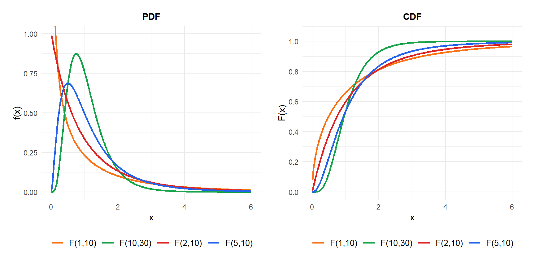
Effect of degrees of freedom
Both \(d_1\) and \(d_2\) affect the shape:
- Small \(d_1\) or \(d_2\): heavily right-skewed with a long tail.
- Large \(d_1\) and \(d_2\): the distribution becomes more symmetric and concentrates near 1 (since both chi-squared variables become approximately equal to their means).
- \(d_1 = 1\): the distribution has a singularity at 0 and decays slowly.
- \(d_2 \to \infty\): \(d_1 \cdot F(d_1, d_2) \to \chi^2(d_1)\).
Properties
For \(X \sim F(d_1, d_2)\):
- Expected Value (Mean)
\[E(X) = \frac{d_2}{d_2 - 2}, \quad \text{for } d_2 > 2\]
The mean is always greater than 1 and approaches 1 as \(d_2 \to \infty\).
- Variance
\[\text{Var}(X) = \frac{2d_2^2(d_1 + d_2 - 2)}{d_1(d_2-2)^2(d_2-4)}, \quad \text{for } d_2 > 4\]
- Skewness
\[\text{Skewness} = \frac{(2d_1 + d_2 - 2)\sqrt{8(d_2-4)}}{(d_2-6)\sqrt{d_1(d_1+d_2-2)}}, \quad \text{for } d_2 > 6\]
Always positive: the F distribution is always right-skewed.
- Mode
\[\text{Mode} = \frac{d_1 - 2}{d_1} \cdot \frac{d_2}{d_2 + 2}, \quad \text{for } d_1 > 2\]
- Quantile Function
No closed form. Critical values are read from F-tables or computed with software. In R: qf(0.95, df1, df2).
Applications
One-way ANOVA
ANOVA tests whether the means of \(k\) groups are all equal. The test statistic is:
\[F = \frac{\text{MS}_{\text{between}}}{\text{MS}_{\text{within}}} = \frac{\text{SS}_{\text{between}}/(k-1)}{\text{SS}_{\text{within}}/(n-k)} \sim F(k-1,\, n-k)\]
under \(H_0: \mu_1 = \mu_2 = \cdots = \mu_k\).
A large \(F\) means between-group variability is much larger than within-group variability, evidence against equal means.
Three fertilizer types are tested on 5 plots each (\(k=3\), \(n=15\)). The ANOVA table gives:
| Source | SS | df | MS | F |
|---|---|---|---|---|
| Between | 84.4 | 2 | 42.2 | 7.34 |
| Within | 69.0 | 12 | 5.75 | |
| Total | 153.4 | 14 |
Critical value: \(F_{0.95}(2, 12) \approx 3.89\).
Since \(7.34 > 3.89\), we reject \(H_0\): at least one fertilizer type produces a different mean yield (\(p \approx 0.008\)).
F-test in regression
In multiple linear regression with \(p\) predictors and \(n\) observations, the overall F-test checks whether any predictor is useful:
\[F = \frac{R^2/p}{(1-R^2)/(n-p-1)} \sim F(p,\, n-p-1)\]
under \(H_0\) that all regression coefficients are zero.
A regression model with \(p = 4\) predictors is fitted to \(n = 50\) observations. The model achieves \(R^2 = 0.62\).
\[F = \frac{0.62/4}{0.38/45} = \frac{0.155}{0.00844} \approx 18.4\]
Critical value: \(F_{0.95}(4, 45) \approx 2.58\).
Since \(18.4 \gg 2.58\), we strongly reject \(H_0\): the model explains a significant proportion of the variance (\(p < 0.001\)).
Test for equality of two variances
To test \(H_0: \sigma_1^2 = \sigma_2^2\) using samples of sizes \(n_1\) and \(n_2\):
\[F = \frac{S_1^2}{S_2^2} \sim F(n_1 - 1,\, n_2 - 1)\]
under \(H_0\). Values far from 1 (in either direction) suggest unequal variances.
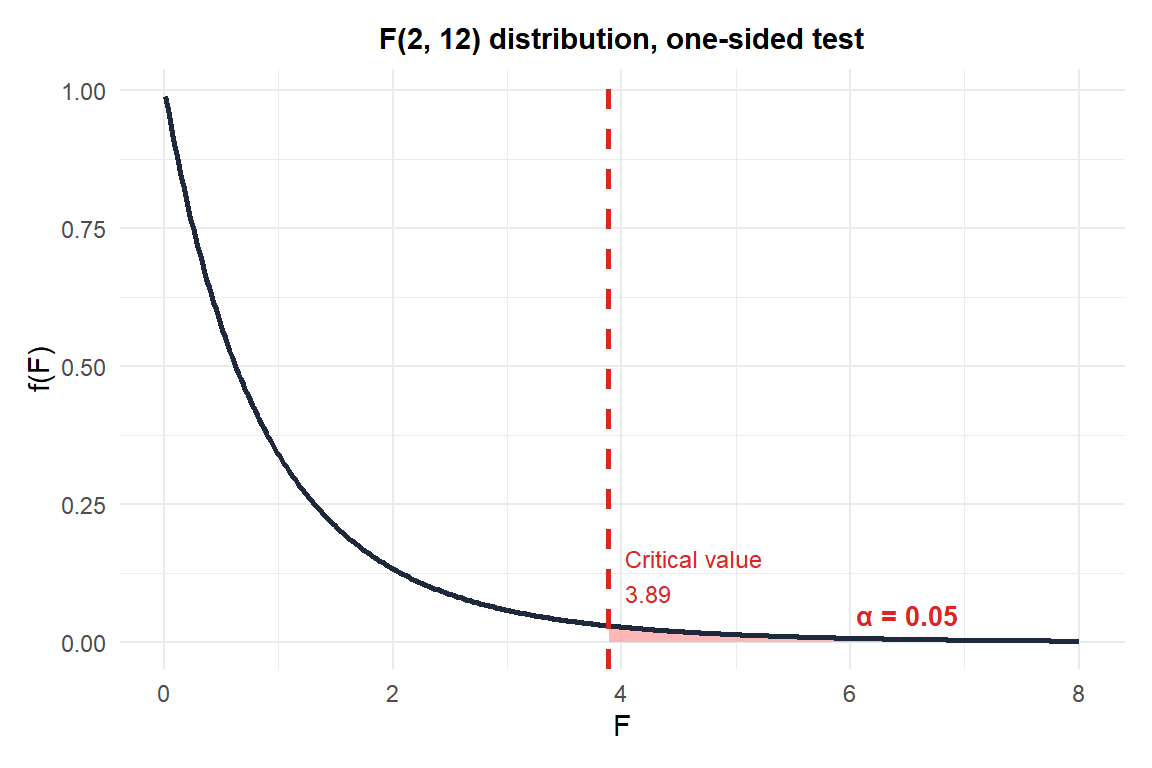
Figure 1: F(2,12) distribution: rejection region at α=0.05 starts at the critical value 3.89
⚠️ The F-test for equal variances is sensitive to non-normality
The variance ratio test \(F = S_1^2/S_2^2\) assumes both populations are normal. It is extremely sensitive to departures from normality: non-normal data can produce a significant result even when variances are equal. For robust alternatives, use Levene’s test or Bartlett’s test, which are less sensitive to the normality assumption.
💡 Relationship with other distributions
- Chi-squared: \(d_1 \cdot F(d_1, d_2) \xrightarrow{d_2\to\infty} \chi^2(d_1)\).
- Student’s t: \(t(\nu)^2 = F(1, \nu)\). Squaring a t statistic gives an F statistic with 1 numerator df.
- Beta: if \(X \sim F(d_1, d_2)\), then \(\frac{d_1 X/d_2}{1 + d_1 X/d_2} \sim \text{Beta}(d_1/2, d_2/2)\).
- Uniform: \(F(2, 2) = \text{Lomax}(1,1)\) (not uniform, but note that \(F(1,1)\) is related to the squared Cauchy).

