Exponential distribution
The exponential distribution models the waiting time between events in a Poisson process. It is the continuous counterpart of the geometric distribution and the only continuous distribution with the memoryless property.
Definition
A random variable \(X\) follows an exponential distribution with rate parameter \(\lambda > 0\), written \(X \sim \text{Exp}(\lambda)\), if its probability density function is:
\[f(x) = \lambda e^{-\lambda x}, \quad x \geq 0\]
The parameter \(\lambda\) is the rate: the average number of events per unit of time. The mean waiting time between events is \(1/\lambda\).
⚠️ Rate vs mean parametrization
The exponential distribution is parametrized in two different ways depending on the source:
- Rate parametrization (\(\lambda\)): \(f(x) = \lambda e^{-\lambda x}\). Mean \(= 1/\lambda\). Used by most probability textbooks and R’s
dexp(x, rate = lambda). - Mean parametrization (\(\theta = 1/\lambda\)): \(f(x) = \frac{1}{\theta} e^{-x/\theta}\). Mean \(= \theta\). Common in reliability engineering and some engineering textbooks.
Always check which convention your source uses. If a problem says “average time between failures is 5 hours”, then \(\theta = 5\) and \(\lambda = 0.2\).
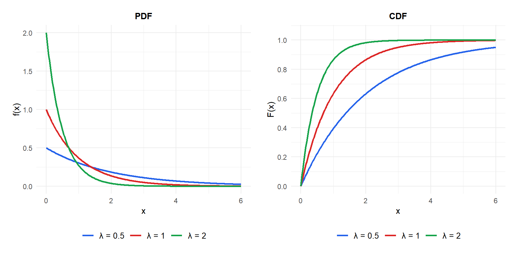
Probability Density Function and CDF
The CDF has a clean closed form:
\[F(x) = P(X \leq x) = 1 - e^{-\lambda x}, \quad x \geq 0\]
The survival function (probability of surviving beyond \(x\)) is simply:
\[P(X > x) = e^{-\lambda x}\]
Properties
For \(X \sim \text{Exp}(\lambda)\):
- Expected Value (Mean)
\[E(X) = \frac{1}{\lambda}\]
- Variance
\[\text{Var}(X) = \frac{1}{\lambda^2}\]
Note that \(\text{SD}(X) = 1/\lambda = E(X)\): the standard deviation equals the mean. This is a distinctive property of the exponential.
- Skewness
Always 2: the exponential is always right-skewed, regardless of \(\lambda\).
- Kurtosis
\[g_2 = 6\]
Strongly leptokurtic: the exponential has much heavier tails than the normal distribution.
- Mode
Always 0: the most likely value is at the origin.
- Quantile Function
\[Q(p) = -\frac{1}{\lambda}\ln(1-p)\]
The median is \(Q(0.5) = \ln(2)/\lambda \approx 0.693/\lambda\), which is less than the mean \(1/\lambda\). The distribution is right-skewed so the median is always below the mean.
The memoryless property
The exponential distribution is the only continuous distribution with the memoryless property:
\[P(X > s + t \mid X > s) = P(X > t)\]
If you have already waited \(s\) units of time without an event occurring, the probability of waiting an additional \(t\) units is exactly the same as if you had just started waiting. Past waiting time provides zero information about the future.
A server has been running for 3 years without failure. Its uptime follows \(\text{Exp}(\lambda)\). What is the probability it runs for at least 2 more years?
By the memoryless property, this is exactly \(P(X > 2) = e^{-2\lambda}\), the same probability you would compute if the server had just been switched on. The 3 years of trouble-free operation are completely irrelevant.
⚠️ When the memoryless property does not hold
The exponential distribution assumes a constant failure rate: a component is equally likely to fail in any given instant regardless of its age. This is realistic for electronic components subject to random external shocks (cosmic rays, power surges), but not for mechanical components that wear out over time. For aging components, the Weibull distribution is more appropriate: it allows the failure rate to increase (or decrease) with age.
Step-by-step example
A data center’s servers fail on average once every 200 days (\(\lambda = 1/200\)). Let \(X\) = days until the next failure, \(X \sim \text{Exp}(1/200)\).
Probability of surviving more than 100 days:
\[P(X > 100) = e^{-100/200} = e^{-0.5} \approx 0.6065\]
About 61% of servers survive beyond 100 days without failure.
Probability of failing within the first 50 days:
\[F(50) = 1 - e^{-50/200} = 1 - e^{-0.25} \approx 0.2212\]
About 22% of servers fail within the first 50 days.
Median time to failure:
\[Q(0.5) = -200\ln(0.5) = 200\ln(2) \approx 138.6 \text{ days}\]
Half of all servers fail before 138.6 days, even though the mean is 200 days. The right skew means the mean is pulled up by the rare very long-lasting servers.
Call center: calls arrive at a rate of 5 per minute (\(\lambda = 5\)). Time between calls: \(\text{Exp}(5)\). Mean wait: \(1/5 = 0.2\) minutes = 12 seconds.
Radioactive decay: a radioactive atom decays with rate \(\lambda = 0.001\) per year. Probability of surviving 500 years: \(e^{-0.5} \approx 0.607\).
Customer service: average call duration is 8 minutes (\(\theta = 8\), \(\lambda = 1/8\)). Probability that a call lasts more than 15 minutes: \(e^{-15/8} \approx 0.153\).
Connection with the Poisson distribution
The exponential and Poisson distributions are two sides of the same model. If events occur according to a Poisson process with rate \(\lambda\):
- The number of events in a fixed interval of length \(t\) follows \(\text{Poisson}(\lambda t)\).
- The waiting time between consecutive events follows \(\text{Exp}(\lambda)\).
This connection means that if you know \(\lambda\) for a Poisson count model, you automatically know the distribution of inter-event times, and vice versa.
💡 Relationship with other distributions
- Geometric: the discrete analogue. Both are memoryless, one for trial counts, the other for continuous time.
- Poisson: if inter-arrival times are \(\text{Exp}(\lambda)\), arrivals follow a \(\text{Poisson}(\lambda)\) process.
- Gamma: the sum of \(k\) independent \(\text{Exp}(\lambda)\) variables follows \(\text{Gamma}(k, \lambda)\).
- Weibull: a generalization of the exponential that allows non-constant failure rates. \(\text{Exp}(\lambda) = \text{Weibull}(1, \lambda)\).

