Continuous uniform distribution
The continuous uniform distribution assigns equal probability density to all values in an interval \((a, b)\). It is the simplest continuous distribution and the mathematical model for “pick a random number between \(a\) and \(b\).”
Definition
A random variable \(X\) follows a continuous uniform distribution on the interval \((a, b)\), written \(X \sim U(a, b)\), if its probability density function (PDF) is:
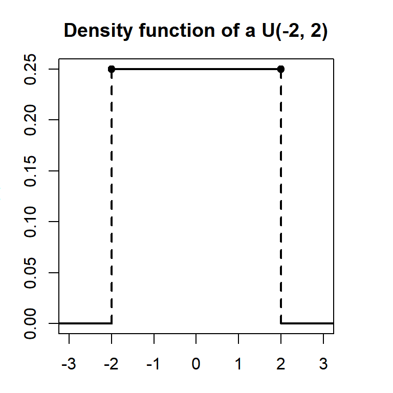
\[f(x) = \begin{cases} \dfrac{1}{b-a} & \text{if } x \in (a, b) \\ 0 & \text{otherwise} \end{cases}\]
The density is constant over the interval: no value is more likely than any other. The height of the rectangle is \(1/(b-a)\), chosen so that the total area equals 1.
⚠️ The PDF can exceed 1
For a \(U(0, 0.1)\) distribution, \(f(x) = 1/0.1 = 10\) everywhere on the interval. This is valid: \(f(x)\) is a density, not a probability, and densities have no upper bound. The probability of any interval is the area under the curve, not the height. The constraint is \(\int_{-\infty}^{\infty} f(x)\,dx = 1\), not \(f(x) \leq 1\).
Cumulative Distribution Function
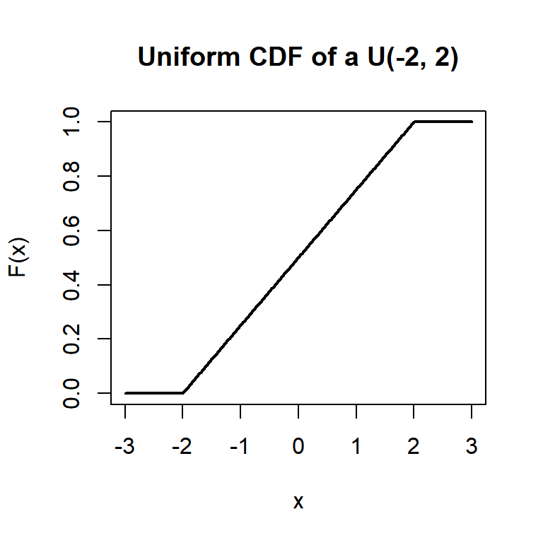
The CDF increases linearly from 0 to 1 across the interval:
\[F(x) = \begin{cases} 0 & \text{if } x < a \\ \dfrac{x-a}{b-a} & \text{if } a \leq x \leq b \\ 1 & \text{if } x > b \end{cases}\]
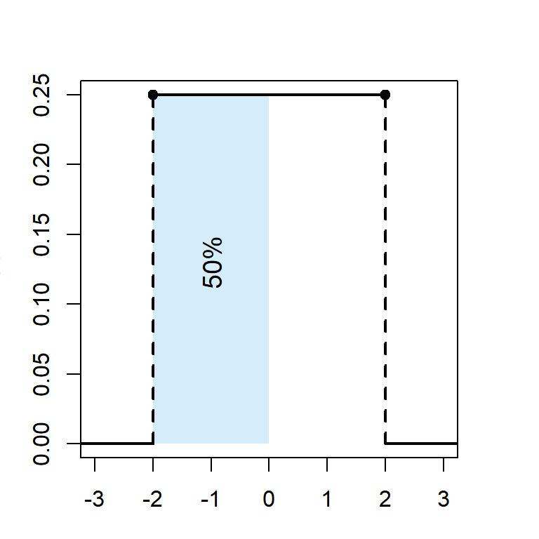
The probability of falling in any sub-interval \([c, d] \subseteq [a, b]\) is simply proportional to its length:
\[P(c \leq X \leq d) = \frac{d - c}{b - a}\]
Properties
For \(X \sim U(a, b)\):
- Expected Value (Mean)
\[E(X) = \frac{a + b}{2}\]
The mean is the midpoint of the interval. Because the distribution is symmetric, mean and median coincide.
- Variance
\[\text{Var}(X) = \frac{(b-a)^2}{12}\]
Variance grows with the square of the interval width: doubling the range quadruples the variance.
- Skewness
Always 0. The distribution is perfectly symmetric around its mean.
- Kurtosis
\[g_2 = -\frac{6}{5} = -1.2\]
Platykurtic: flatter than the normal distribution with lighter tails.
- Mode
Any value in \((a, b)\) is a mode: the density is constant, so no single value is more likely than any other.
- Quantile Function
\[Q(p) = a + p(b - a)\]
A linear interpolation between \(a\) and \(b\). The median is \(Q(0.5) = (a+b)/2\).
Step-by-step example
A delivery service guarantees arrival within a 2-hour window. The actual arrival time \(X\) is uniformly distributed, \(X \sim U(0, 120)\) minutes.
Probability of arriving in the first 30 minutes:
\[P(X \leq 30) = F(30) = \frac{30 - 0}{120 - 0} = 0.25\]
Probability of arriving between 45 and 90 minutes:
\[P(45 \leq X \leq 90) = \frac{90 - 45}{120} = \frac{45}{120} = 0.375\]
Expected arrival time:
\[E(X) = \frac{0 + 120}{2} = 60 \text{ minutes}\]
Variance and standard deviation:
\[\text{Var}(X) = \frac{120^2}{12} = 1200, \qquad \text{SD}(X) = \sqrt{1200} \approx 34.6 \text{ minutes}\]
- Round-off error: when a measurement is rounded to the nearest integer, the rounding error is \(U(-0.5, 0.5)\). Expected error: 0. Variance: \(1/12 \approx 0.083\).
- Random number generation: computer random number generators produce \(U(0, 1)\) values, which are then transformed to any other distribution.
- Bus waiting time: if buses run every 10 minutes and you arrive at a random time, your wait is \(U(0, 10)\). Expected wait: 5 minutes.
The inverse transform method
The \(U(0, 1)\) distribution is the foundation of simulation. The inverse transform method states: if \(U \sim U(0, 1)\), then \(X = F^{-1}(U)\) follows any distribution with CDF \(F\).
For the uniform on \((a, b)\): \(X = a + U(b - a)\). For an exponential with rate \(\lambda\): \(X = -\ln(U)/\lambda\). This is how most statistical software generates random numbers from any distribution.
💡 Relationship with other distributions
- Discrete uniform: the continuous uniform is the continuous analogue. Both assign equal probability to all outcomes.
- Beta distribution: \(U(0,1)\) is a special case of \(\text{Beta}(1, 1)\).
- Order statistics: the \(k\)-th order statistic of \(n\) independent \(U(0,1)\) variables follows a \(\text{Beta}(k, n-k+1)\) distribution.
- Simulation: every random number generator starts with \(U(0,1)\) and transforms it into the target distribution using the quantile function.

