Beta distribution
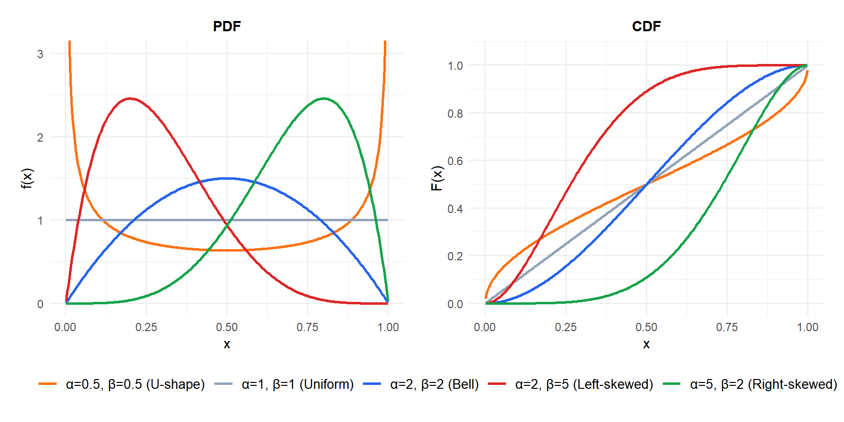
The beta distribution is defined on the interval \([0, 1]\) and is extraordinarily flexible: depending on its two shape parameters, it can take almost any shape: uniform, bell-shaped, U-shaped, J-shaped, or skewed in either direction. This makes it the natural model for proportions, probabilities, and rates.
Definition
A random variable \(X\) follows a beta distribution with shape parameters \(\alpha > 0\) and \(\beta > 0\), written \(X \sim \text{Beta}(\alpha, \beta)\), if:
\[f(x) = \frac{x^{\alpha-1}(1-x)^{\beta-1}}{B(\alpha, \beta)}, \quad 0 \leq x \leq 1\]
where \(B(\alpha, \beta) = \frac{\Gamma(\alpha)\Gamma(\beta)}{\Gamma(\alpha+\beta)}\) is the beta function, which acts as a normalizing constant ensuring the PDF integrates to 1.
The CDF has no closed form for general \(\alpha, \beta\) and is computed numerically as the regularized incomplete beta function \(I_x(\alpha, \beta)\).
⚠️ The beta function vs the beta distribution
The beta function \(B(\alpha, \beta)\) is a mathematical function used as the normalizing constant in the PDF. It is not the same as the beta distribution. The beta distribution is a probability distribution; the beta function is a special function. Both use the same Greek letters, which causes confusion in textbooks.
How the shape parameters control the distribution
The behavior of the beta distribution changes dramatically depending on \(\alpha\) and \(\beta\):
- \(\alpha = \beta = 1\): uniform distribution on \([0,1]\).
- \(\alpha = \beta > 1\): symmetric bell shape centered at 0.5. Larger values give a narrower bell.
- \(\alpha = \beta < 1\): U-shaped, with probability concentrated near 0 and 1.
- \(\alpha > \beta\): right-skewed, distribution leans toward 1.
- \(\alpha < \beta\): left-skewed, distribution leans toward 0.
- \(\alpha > 1\), \(\beta = 1\): power function distribution, monotonically increasing.
- \(\alpha = 1\), \(\beta > 1\): monotonically decreasing.
Properties
For \(X \sim \text{Beta}(\alpha, \beta)\):
- Expected Value (Mean)
\[E(X) = \frac{\alpha}{\alpha + \beta}\]
- Variance
\[\text{Var}(X) = \frac{\alpha\beta}{(\alpha+\beta)^2(\alpha+\beta+1)}\]
- Skewness
\[\text{Skewness} = \frac{2(\beta - \alpha)\sqrt{\alpha+\beta+1}}{(\alpha+\beta+2)\sqrt{\alpha\beta}}\]
Positive when \(\alpha < \beta\) (left-skewed toward 0), negative when \(\alpha > \beta\) (right-skewed toward 1), zero when \(\alpha = \beta\).
- Kurtosis
\[g_2 = \frac{6\left[(\alpha-\beta)^2(\alpha+\beta+1) - \alpha\beta(\alpha+\beta+2)\right]}{\alpha\beta(\alpha+\beta+2)(\alpha+\beta+3)}\]
- Mode
\[\text{Mode} = \frac{\alpha - 1}{\alpha + \beta - 2}, \quad \text{for } \alpha > 1 \text{ and } \beta > 1\]
For \(\alpha \leq 1\) or \(\beta \leq 1\), the mode is at 0, 1, or both endpoints (U-shape).
- Quantile Function
No closed form; computed numerically via the inverse incomplete beta function.
The beta distribution as a Bayesian prior
The beta distribution is the conjugate prior for the binomial likelihood. This means: if you observe \(k\) successes in \(n\) Bernoulli trials and your prior belief about the success probability \(p\) is \(\text{Beta}(\alpha, \beta)\), then your updated (posterior) belief is:
\[p \mid k,n \sim \text{Beta}(\alpha + k,\ \beta + n - k)\]
The posterior is still a beta distribution, just with updated parameters. The parameters \(\alpha\) and \(\beta\) in the prior can be interpreted as pseudo-counts: \(\alpha - 1\) prior successes and \(\beta - 1\) prior failures.
A conversion rate optimizer wants to estimate the click-through rate \(p\) of a new button design. Before seeing any data, they assume \(p \sim \text{Beta}(1, 1)\) (uniform prior: all rates equally plausible).
After showing the button to 100 visitors, 12 click it. The posterior is:
\[p \mid \text{data} \sim \text{Beta}(1 + 12,\ 1 + 88) = \text{Beta}(13, 89)\]
Posterior mean: \(13/(13+89) \approx 0.127\).
Posterior mode: \((13-1)/(13+89-2) = 12/100 = 0.12\) (same as the MLE).
A 95% credible interval: qbeta(c(0.025, 0.975), 13, 89) \(\approx (0.067, 0.208)\).
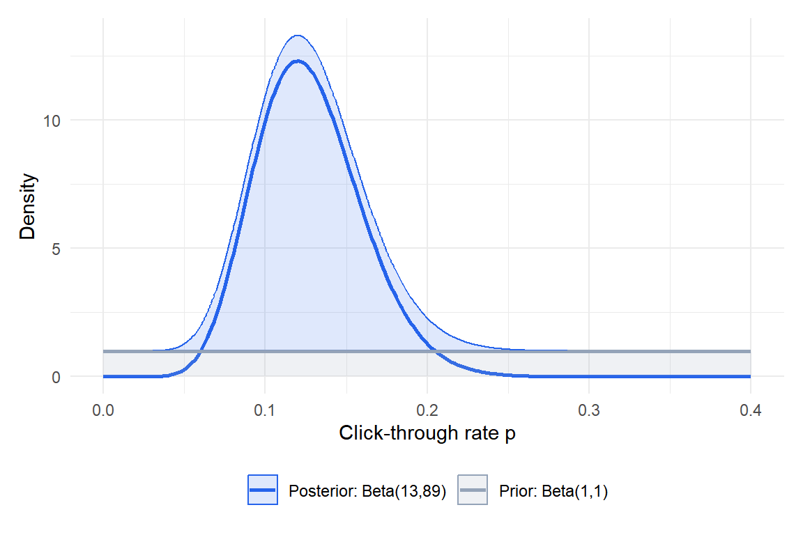
Figure 1: Bayesian updating: flat prior Beta(1,1) updated to Beta(13,89) after observing 12 clicks out of 100 visitors
Step-by-step example
A manufacturing process has a defect rate \(p\) that is modeled as \(p \sim \text{Beta}(3, 15)\), based on historical data suggesting most batches have a defect rate around 15-20%.
Expected defect rate:
\[E(p) = \frac{3}{3+15} = \frac{3}{18} \approx 0.167\]
Variance:
\[\text{Var}(p) = \frac{3 \times 15}{18^2 \times 19} \approx 0.0073\]
Standard deviation \(\approx 0.086\).
Mode (most likely defect rate):
\[\text{Mode} = \frac{3-1}{3+15-2} = \frac{2}{16} = 0.125\]
Probability that the defect rate exceeds 25%:
\[P(p > 0.25) = 1 - F(0.25) = 1 - I_{0.25}(3, 15) \approx 1 - 0.902 = 0.098\]
About 10% of batches have a defect rate above 25%.
A/B test: after a test, conversion rates for two variants are modeled as \(p_A \sim \text{Beta}(40, 160)\) and \(p_B \sim \text{Beta}(55, 145)\). The probability that \(p_B > p_A\) can be computed by simulation or numerical integration - this is the core of Bayesian A/B testing.
Project completion rate: in project management, the fraction of tasks completed on time in similar projects follows \(\text{Beta}(8, 2)\) (mean 0.8, most projects complete 80%+ on time). Probability of completing more than 90% on time: \(P(X > 0.9) = 1 - I_{0.9}(8,2) \approx 0.264\).
Order statistics: the \(k\)-th order statistic of \(n\) independent \(\text{Uniform}(0,1)\) variables follows \(\text{Beta}(k, n-k+1)\).
💡 Relationship with other distributions
- Uniform: \(\text{Beta}(1,1) = \text{Uniform}(0,1)\).
- Gamma: if \(X \sim \text{Gamma}(\alpha,1)\) and \(Y \sim \text{Gamma}(\beta,1)\) independently, then \(X/(X+Y) \sim \text{Beta}(\alpha,\beta)\).
- Binomial: the beta is the conjugate prior for the binomial likelihood parameter \(p\).
- Dirichlet: the multivariate generalization of the beta distribution, used for modeling probability vectors (e.g. topic distributions in text models).
- Order statistics: \(\text{Beta}(k, n-k+1)\) is the distribution of the \(k\)-th order statistic from \(n\) uniform samples.

