Pearson's chi-squared test
Pearson’s chi-squared test determines whether two categorical variables are associated or whether their distribution across categories is what we would expect by chance. It is one of the most widely used tests in statistics, appearing in everything from clinical trials to market research.
What is Pearson’s chi-squared test?
When you have two categorical variables and want to know whether they are related, the chi-squared test is the standard tool. The idea is simple: if there is no association between the variables, the distribution of one variable should be roughly the same across all categories of the other. The test compares what you actually observed with what you would expect to see under that assumption of independence.
The test statistic is:
\[ \chi^2 = \sum_{i} \frac{(O_i - E_i)^2}{E_i} \]
where \(O_i\) is the observed frequency in cell \(i\) and \(E_i\) is the expected frequency under the null hypothesis of independence.
Under the null hypothesis, this statistic follows a chi-squared distribution with degrees of freedom:
\[df = (r - 1)(c - 1)\]
where \(r\) is the number of rows and \(c\) is the number of columns in the contingency table.
Hypotheses
- \(H_0\): the two variables are independent (no association).
- \(H_1\): the two variables are associated.
The test is always one-sided in the sense that large values of \(\chi^2\) (when observed frequencies are very different from expected) lead to rejection of \(H_0\).
Expected frequencies
Under the null hypothesis of independence, the expected frequency for each cell is:
\[E_{ij} = \frac{\text{Row total}_i \times \text{Column total}_j}{n}\]
where \(n\) is the total sample size. This formula comes directly from the definition of independence in probability: if \(X\) and \(Y\) are independent, \(P(X = i, Y = j) = P(X = i) \cdot P(Y = j)\).
Step-by-step example
A public health study collects data on 200 individuals, recording their smoking status and whether they developed lung cancer:
| Lung Cancer: Yes | Lung Cancer: No | Row total | |
|---|---|---|---|
| Smoker | 70 | 30 | 100 |
| Non-smoker | 20 | 80 | 100 |
| Column total | 90 | 110 | 200 |
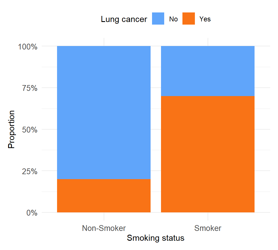
Figure 1: Observed frequencies: smokers show a much higher proportion of lung cancer cases than non-smokers
Step 1: calculate expected frequencies.
\[E_{11} = \frac{100 \times 90}{200} = 45, \quad E_{12} = \frac{100 \times 110}{200} = 55\]
\[E_{21} = \frac{100 \times 90}{200} = 45, \quad E_{22} = \frac{100 \times 110}{200} = 55\]
| Cancer: Yes | Cancer: No | |
|---|---|---|
| Smoker | \(O=70\), \(E=45\) | \(O=30\), \(E=55\) |
| Non-smoker | \(O=20\), \(E=45\) | \(O=80\), \(E=55\) |
Step 2: calculate the test statistic.
\[\chi^2 = \frac{(70-45)^2}{45} + \frac{(30-55)^2}{55} + \frac{(20-45)^2}{45} + \frac{(80-55)^2}{55}\]
\[\chi^2 = \frac{625}{45} + \frac{625}{55} + \frac{625}{45} + \frac{625}{55} = 13.89 + 11.36 + 13.89 + 11.36 = 50.50\]
Step 3: determine degrees of freedom and critical value.
\[df = (2-1)(2-1) = 1\]
For \(df = 1\) and a significance level of \(\alpha = 0.05\), the critical value is \(\chi^2_{0.05, 1} = 3.84\).
Step 4: conclusion.
Since \(50.50 \gg 3.84\), we reject \(H_0\). There is strong statistical evidence of an association between smoking status and lung cancer incidence.
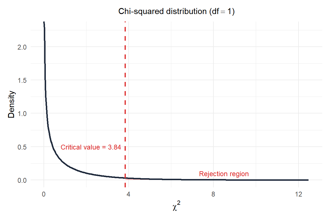
Figure 2: Chi-squared distribution with 1 df: the observed statistic (50.5) falls far into the rejection region
A second example: product preference by gender
A marketing team surveys 150 customers about their preferred product (A, B, or C), split by gender:
| Product A | Product B | Product C | Total | |
|---|---|---|---|---|
| Male | 30 | 25 | 20 | 75 |
| Female | 20 | 35 | 20 | 75 |
| Total | 50 | 60 | 40 | 150 |
Expected frequencies (e.g. \(E_{11} = 75 \times 50 / 150 = 25\)):
| Product A | Product B | Product C | |
|---|---|---|---|
| Male | 25 | 30 | 20 |
| Female | 25 | 30 | 20 |
\[\chi^2 = \frac{(30-25)^2}{25} + \frac{(25-30)^2}{30} + \frac{(20-20)^2}{20} + \frac{(20-25)^2}{25} + \frac{(35-30)^2}{30} + \frac{(20-20)^2}{20}\]
\[\chi^2 = 1.00 + 0.83 + 0 + 1.00 + 0.83 + 0 = 3.67\]
\[df = (2-1)(3-1) = 2, \quad \chi^2_{0.05,\, 2} = 5.99\]
Since \(3.67 < 5.99\), we fail to reject \(H_0\). There is no significant evidence that product preference depends on gender in this sample.
Failing to reject the null hypothesis does not mean the variables are definitely independent. It means the data does not provide enough evidence to conclude they are associated, given the sample size and significance level chosen. With a larger sample, the same pattern of differences might become statistically significant.
Assumptions and limitations
⚠️ The expected frequency rule: minimum of 5 per cell
Pearson’s chi-squared test requires that all expected frequencies are at least 5. If any cell has an expected frequency below 5, the chi-squared approximation breaks down and the p-value becomes unreliable. In that case, use Fisher’s exact test instead, which is valid for any sample size and is the standard choice for small samples or sparse tables.
Other assumptions to check:
- Independence of observations: each individual must appear in exactly one cell. Paired or repeated-measures data require different tests.
- Random sampling: the data should come from a random sample of the population of interest.
- Categorical variables: chi-squared works with nominal or ordinal categories, not with continuous measurements.
⚠️ Association is not causation
A significant chi-squared test tells you the two variables are associated in your sample. It says nothing about the direction of the effect, the size of the effect, or whether one variable causes the other. In the smoking and lung cancer example, the test confirms association but the causal link requires much stronger evidence from study design, not from the test statistic alone.
💡 Measuring the strength of the association
The chi-squared statistic tells you whether an association exists, but not how strong it is. For 2×2 tables, use Phi (\(\phi\)): $ = $, which ranges from 0 to 1. For larger tables, use Cramér’s V: $ V = $. Both measure effect size independently of sample size.

