Pearson correlation coefficient
The Pearson correlation coefficient measures the strength and direction of the linear relationship between two quantitative variables. It is one of the most used statistics in research, and one of the most misinterpreted.
Definition
The Pearson correlation coefficient \(r\) is a standardized measure of linear association between two variables \(X\) and \(Y\). It always falls between \(-1\) and \(1\):
- \(r = 1\): perfect positive linear relationship.
- \(r = -1\): perfect negative linear relationship.
- \(r = 0\): no linear relationship.
The formula expresses \(r\) as the ratio of the covariance to the product of the standard deviations:
\[ r = \frac{\sum_{i=1}^{n}(x_i - \bar{x})(y_i - \bar{y})}{\sqrt{\sum_{i=1}^{n}(x_i - \bar{x})^2 \cdot \sum_{i=1}^{n}(y_i - \bar{y})^2}} \]
This is equivalent to:
\[r = \frac{s_{XY}}{s_X \cdot s_Y}\]
where \(s_{XY}\) is the sample covariance, and \(s_X\), \(s_Y\) are the sample standard deviations. Dividing by the standard deviations removes the units, making \(r\) dimensionless and directly comparable across datasets.
Interpreting the value of r
The sign tells you the direction; the absolute value tells you the strength:
| Value of \(\|r\|\) | Interpretation |
|---|---|
| \(0.9 - 1.0\) | Very strong |
| \(0.7 - 0.9\) | Strong |
| \(0.5 - 0.7\) | Moderate |
| \(0.3 - 0.5\) | Weak |
| \(0.0 - 0.3\) | Very weak or negligible |
These thresholds are guidelines, not rules. What counts as a “strong” correlation depends heavily on the field: in physics, \(r = 0.7\) might be disappointing; in psychology or social sciences, it can be remarkable.
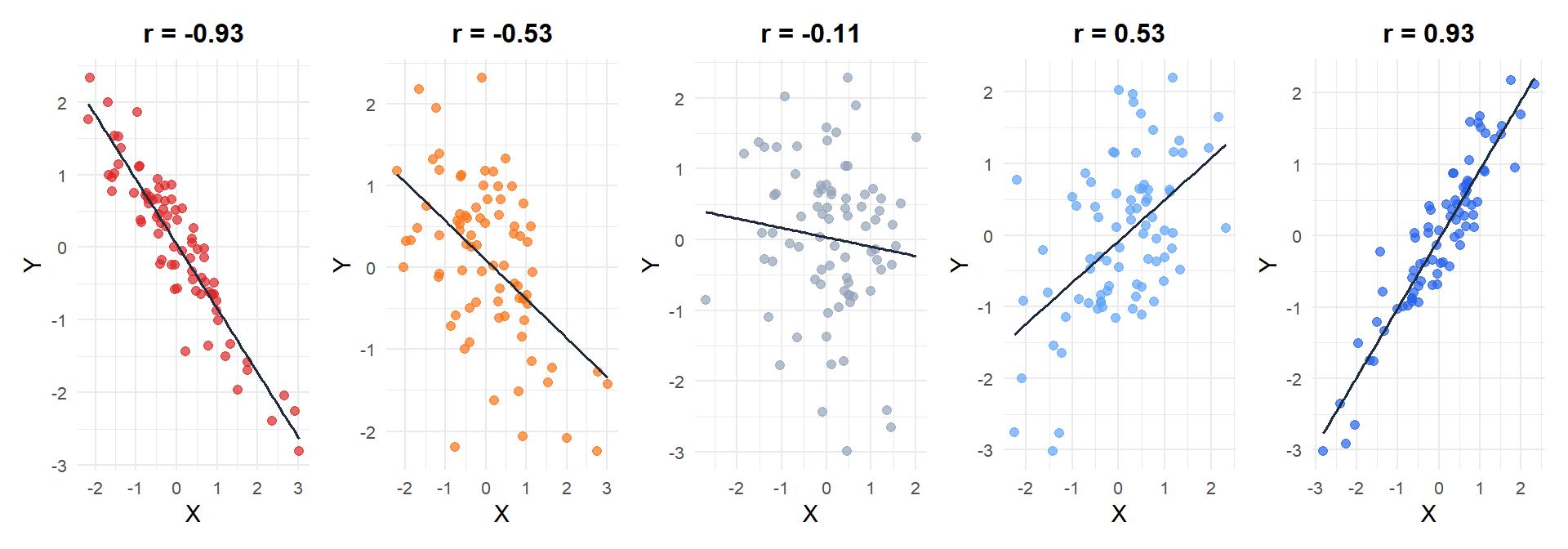
Figure 1: From left to right: strong negative, weak negative, no correlation, weak positive, and strong positive linear relationship
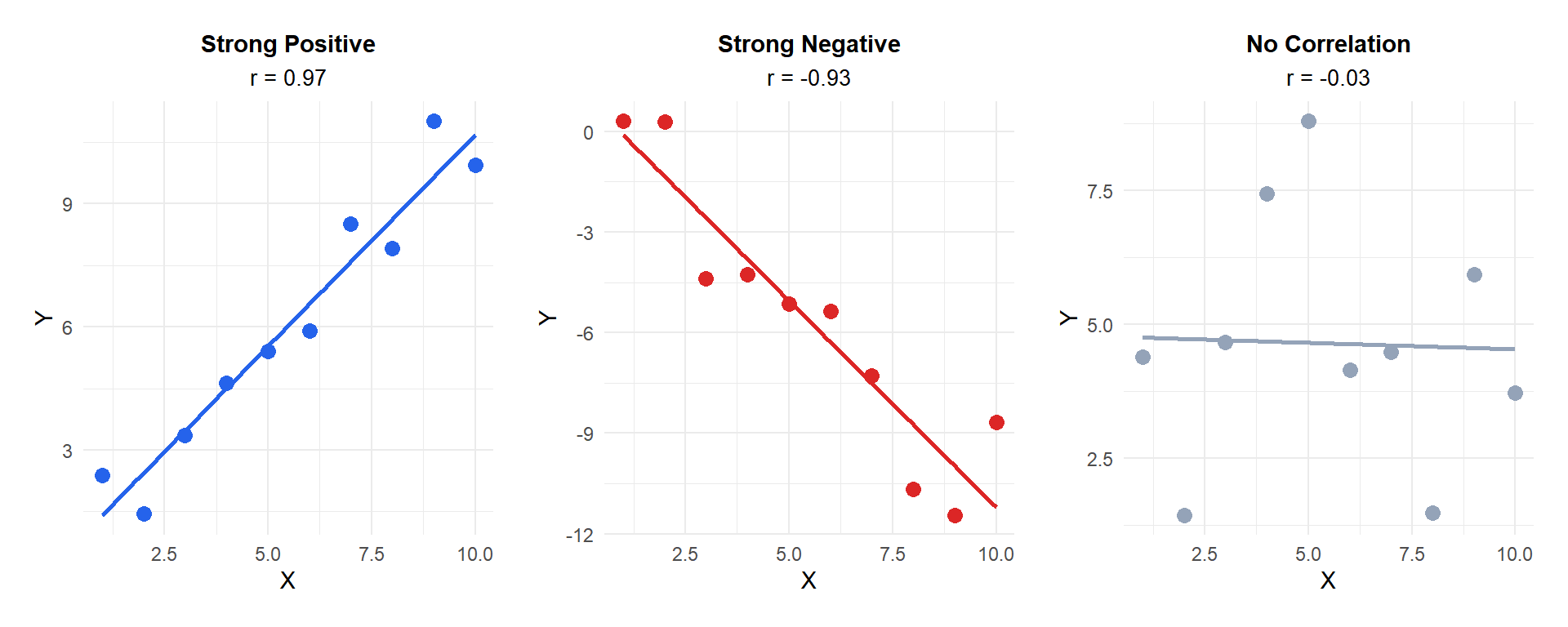
Figure 2: Direction of the linear relationship: positive, negative and no correlation
Step-by-step example
A teacher records the hours studied and exam scores for five students:
| Student | Hours (\(X\)) | Score (\(Y\)) |
|---|---|---|
| 1 | 2 | 50 |
| 2 | 3 | 60 |
| 3 | 5 | 80 |
| 4 | 7 | 85 |
| 5 | 9 | 95 |
Step 1: calculate the means.
\[\bar{x} = \frac{2+3+5+7+9}{5} = 5.2, \quad \bar{y} = \frac{50+60+80+85+95}{5} = 74\]
Step 2: calculate deviations and their products.
| \(x_i\) | \(y_i\) | \(x_i-\bar{x}\) | \(y_i-\bar{y}\) | \((x_i-\bar{x})(y_i-\bar{y})\) | \((x_i-\bar{x})^2\) | \((y_i-\bar{y})^2\) |
|---|---|---|---|---|---|---|
| 2 | 50 | \(-3.2\) | \(-24\) | \(76.8\) | \(10.24\) | \(576\) |
| 3 | 60 | \(-2.2\) | \(-14\) | \(30.8\) | \(4.84\) | \(196\) |
| 5 | 80 | \(-0.2\) | \(6\) | \(-1.2\) | \(0.04\) | \(36\) |
| 7 | 85 | \(1.8\) | \(11\) | \(19.8\) | \(3.24\) | \(121\) |
| 9 | 95 | \(3.8\) | \(21\) | \(79.8\) | \(14.44\) | \(441\) |
| Sum | \(206.0\) | \(32.80\) | \(1370\) |
Step 3: apply the formula.
\[r = \frac{206.0}{\sqrt{32.80 \times 1370}} = \frac{206.0}{\sqrt{44936}} = \frac{206.0}{212.0} \approx 0.97\]
A correlation of \(0.97\) indicates a very strong positive linear relationship: students who study more hours consistently score higher on the exam.
The coefficient of determination \(r^2\)
Squaring the correlation coefficient gives \(r^2\), the coefficient of determination. It represents the proportion of variance in \(Y\) that is explained by \(X\):
\[r^2 = 0.97^2 \approx 0.94\]
In this example, 94% of the variability in exam scores can be explained by hours studied. The remaining 6% is due to other factors not captured in the model.
💡 r vs r²: which one to report?
Limitations
Correlation is not causation
⚠️ The most common misinterpretation in statistics
A high correlation between two variables does not mean one causes the other. Ice cream sales and drowning rates are positively correlated, but ice cream does not cause drowning: both are driven by hot weather. Nicolas Cage film releases correlate with swimming pool drownings. Per capita cheese consumption correlates with deaths by bedsheet tangling. These are called spurious correlations, and they are embarrassingly easy to find in large datasets. Always think about the mechanism before inferring causality from correlation.
Only detects linear relationships
Pearson’s \(r\) measures linear association only. A strong non-linear relationship can produce \(r \approx 0\).
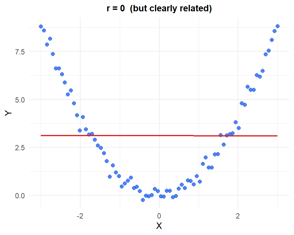
Figure 3: A perfect quadratic relationship gives r ≈ 0: Pearson’s r completely misses non-linear patterns
For non-linear relationships, consider Spearman’s rank correlation or other non-parametric measures.
Sensitivity to outliers
A single extreme observation can dramatically change \(r\). Always inspect the scatter plot before trusting the correlation coefficient.
⚠️ Always plot before computing r
Two datasets can have nearly identical correlation coefficients but completely different scatter plot patterns. This is known as Anscombe’s quartet: four datasets with (r \approx 0.82) that look nothing alike when plotted. Computing (r) without looking at the data is one of the most common analytical mistakes.

