Coefficient of kurtosis in statistics
Kurtosis measures how heavy the tails of a distribution are compared to a normal distribution. While skewness tells you about asymmetry, kurtosis tells you about the likelihood of extreme values: distributions with high kurtosis produce outliers more often than you would expect from a normal curve.
What is kurtosis?
Kurtosis quantifies the concentration of data in the tails versus the center of a distribution. A high kurtosis means more data in the tails and a sharper peak. A low kurtosis means lighter tails and a flatter peak.
The standard formula for the excess kurtosis (the version used by most software, including R) is:
\[ g_2 = \frac{n(n+1)}{(n-1)(n-2)(n-3)} \sum_{i=1}^{n} \left(\frac{x_i - \bar{x}}{s}\right)^4 - \frac{3(n-1)^2}{(n-2)(n-3)} \]
where \(n\) is the number of observations, \(\bar{x}\) is the mean, and \(s\) is the sample standard deviation.
The subtracted term ensures that a normal distribution has \(g_2 = 0\). This is called excess kurtosis: it measures kurtosis relative to the normal distribution, not in absolute terms.
⚠️ Raw kurtosis vs excess kurtosis
There are two versions of the kurtosis formula. Raw kurtosis (without the correction term) gives a value of 3 for a normal distribution. Excess kurtosis subtracts 3 so that the normal distribution gives 0. Most software, including R’s kurtosis() function from the moments package, returns excess kurtosis. Always check which version your software uses before interpreting results.
Types of kurtosis
Mesokurtic (\(g_2 \approx 0\))
The normal distribution is the reference: \(g_2 = 0\). Tails and peak are neither heavy nor light. Most parametric tests assume the data comes from a mesokurtic (or at least approximately normal) distribution.
Leptokurtic (\(g_2 > 0\))
Heavier tails and a sharper peak than normal. More data concentrates near the mean and in the extreme tails, with less in the shoulders. This means outliers are more likely than in a normal distribution.
Real examples: financial asset returns, insurance claims, earthquake magnitudes. The Student’s \(t\)-distribution with low degrees of freedom is leptokurtic.
Platykurtic (\(g_2 < 0\))
Lighter tails and a flatter peak than normal. Data is more evenly spread, with fewer extreme values. The uniform distribution is the classic example.
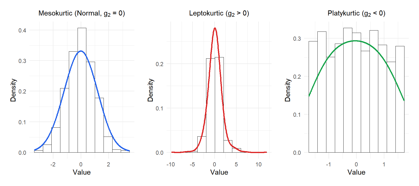
Figure 1: Leptokurtic distributions have heavier tails and a sharper peak than the normal (mesokurtic); platykurtic have lighter tails and a flatter peak
⚠️ High kurtosis is not the same as high variance
A common misconception is that a leptokurtic distribution is simply “more spread out.” It is not. Two distributions can have the same variance and very different kurtosis. What changes is where the variance comes from: in a leptokurtic distribution, most variance comes from rare but extreme observations, not from the bulk of the data. This is why kurtosis matters so much in risk management.
Interpretation guide
| Value of \(g_2\) | Type | Tail behavior |
|---|---|---|
| \(g_2 \approx 0\) | Mesokurtic | Normal tails |
| \(g_2 > 0\) | Leptokurtic | Heavy tails, more outliers |
| \(g_2 < 0\) | Platykurtic | Light tails, fewer outliers |
| \(g_2 > 1\) | Strongly leptokurtic | Outliers much more likely than in normal |
As with skewness, always pair the coefficient with a visual inspection of the distribution.
Step-by-step example
Consider the dataset: \(2, 3, 5, 6, 9, 11, 14, 15, 18, 20\).
Step 1: calculate the mean.
\[\bar{x} = \frac{2+3+5+6+9+11+14+15+18+20}{10} = 10.3\]
Step 2: calculate the sample standard deviation.
\[s = \sqrt{\frac{\sum_{i=1}^{10}(x_i - 10.3)^2}{9}} \approx 6.33\]
Step 3: calculate the fourth standardized deviations.
| \(x_i\) | \(x_i - \bar{x}\) | \(\left(\frac{x_i-\bar{x}}{s}\right)^4\) |
|---|---|---|
| 2 | \(-8.3\) | \(2.889\) |
| 3 | \(-7.3\) | \(1.748\) |
| 5 | \(-5.3\) | \(0.494\) |
| 6 | \(-4.3\) | \(0.211\) |
| 9 | \(-1.3\) | \(0.002\) |
| 11 | \(0.7\) | \(0.000\) |
| 14 | \(3.7\) | \(0.086\) |
| 15 | \(4.7\) | \(0.193\) |
| 18 | \(7.7\) | \(0.878\) |
| 20 | \(9.7\) | \(2.211\) |
| Sum | \(8.712\) |
Step 4: apply the formula.
\[g_2 = \frac{10 \times 11}{9 \times 8 \times 7} \times 8.712 - \frac{3 \times 81}{56} = \frac{110}{504} \times 8.712 - 4.339 \approx 1.901 - 4.339 \approx -1.80\]
The excess kurtosis is approximately \(-1.80\): the distribution is platykurtic, with lighter tails than a normal distribution. The data is spread fairly uniformly between 2 and 20, with no extreme outliers pulling the tails.
Where kurtosis matters
- Finance and risk management: financial returns are well known to be leptokurtic (“fat tails”). Models that assume normality, like classic Black-Scholes, underestimate the probability of extreme losses. The 2008 financial crisis was partly a consequence of ignoring tail risk in return distributions.
- Quality control: a leptokurtic defect distribution signals that most products are fine but a small number are catastrophically defective. A platykurtic one suggests defects are spread evenly, which points to a different type of process problem.
- Testing normality: both skewness and kurtosis are used in formal normality tests such as the Jarque-Bera test, which combines both into a single statistic.
💡 Skewness and kurtosis together: the Jarque-Bera test

