Uniform bootstrap
The uniform bootstrap - also called the nonparametric bootstrap or naive bootstrap - is the standard form of bootstrap resampling. Each observation in the original sample receives equal probability \(1/n\) of being drawn at each step, so the bootstrap samples are drawn from the empirical distribution \(\hat{F}_n\). It is the method described in Efron’s original 1979 paper and the default in most software.
Definition
Given an original sample \(\mathbf{x} = (x_1, \ldots, x_n)\), the uniform bootstrap generates resamples by drawing \(n\) observations independently and with replacement, each chosen uniformly at random from \(\{x_1, \ldots, x_n\}\).
This is equivalent to sampling from the empirical distribution \(\hat{F}_n\), which places probability mass \(1/n\) on each observed value:
\[\hat{F}_n(x) = \frac{1}{n} \sum_{i=1}^n \mathbf{1}(x_i \leq x)\]
The “uniform” in the name refers to the uniform weights \(w_i = 1/n\) assigned to each observation. This distinguishes it from the smoothed bootstrap (which adds noise to the resampled values) and the parametric bootstrap (which samples from a fitted parametric distribution).
The multinomial weight representation
Each bootstrap resample can be characterized by a weight vector \((m_1, m_2, \ldots, m_n)\), where \(m_i\) is the number of times observation \(x_i\) appears in the resample. These counts follow a multinomial distribution:
\[(m_1, m_2, \ldots, m_n) \sim \text{Multinomial}\!\left(n;\; \frac{1}{n}, \frac{1}{n}, \ldots, \frac{1}{n}\right)\]
This means:
- \(E[m_i] = 1\): on average, each observation appears once.
- \(\text{Var}(m_i) = (n-1)/n \approx 1\) for large \(n\).
- About \(1 - (1-1/n)^n \approx 1 - e^{-1} \approx 63.2\%\) of observations appear at least once in any given bootstrap resample. The remaining \(\approx 36.8\%\) are left out.
The out-of-bag (OOB) observations - those not included in a resample - can be used for model validation without a separate test set, which is a key property exploited in random forests and bagged estimators.
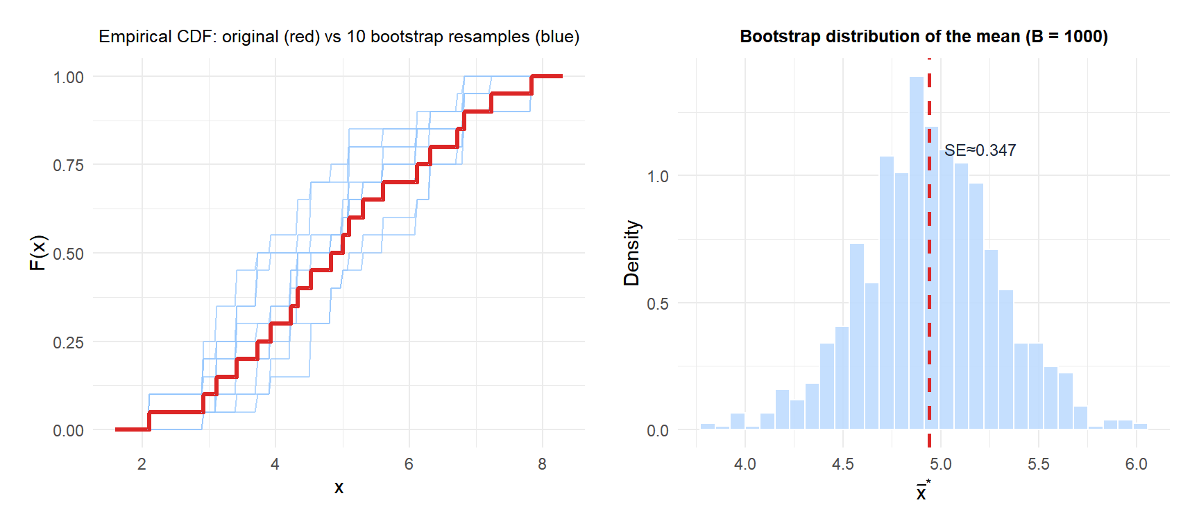
The left panel shows how each bootstrap ECDF (blue) fluctuates around the original ECDF (red): this variability is exactly what the bootstrap uses to estimate uncertainty. The right panel shows the resulting bootstrap distribution of the sample mean.
Complete example
A reliability engineer records the time to failure (hours) of 15 electronic components:
\[x = (120, 95, 142, 108, 87, 155, 131, 99, 167, 113, 78, 144, 102, 138, 91)\]
The observed mean is \(\bar{x} = 117.9\) hours. The theoretical SE of the mean for an exponential distribution would require knowing the rate parameter. Instead, use the uniform bootstrap.
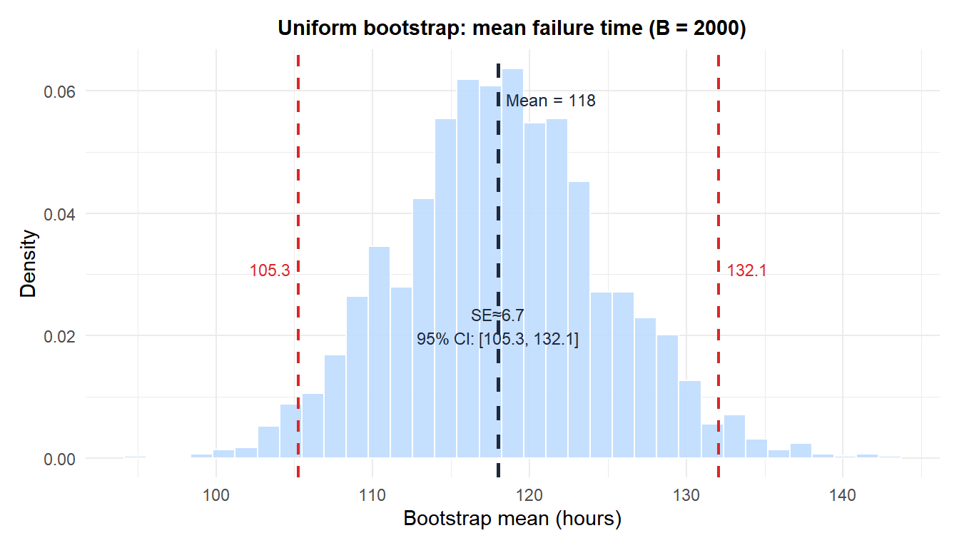
Bootstrap SE \(\approx\) 6.6 hours. The percentile 95% CI gives the bounds shown in red.
Uniform vs other bootstrap variants
| Uniform | Smoothed | Parametric | |
|---|---|---|---|
| Resamples from | \(\hat{F}_n\) (empirical) | \(\hat{F}_n\) + noise | Fitted \(F_\theta\) |
| Assumes distribution | No | No | Yes |
| Handles small \(n\) | Moderate | Better | Best (if correct) |
| Handles continuous data | Discretizes | Correct | Correct |
| Default in practice | Yes | Rarely | Common in modelling |
The uniform bootstrap is the default because it requires no assumptions. Its main weakness is that the empirical distribution \(\hat{F}_n\) is discrete even when the population is continuous, which can underestimate variability in small samples. The smoothed bootstrap addresses this.
💡 The 63.2% rule and out-of-bag estimation
In any uniform bootstrap resample, approximately \(1 - e^{-1} \approx 63.2\%\) of the original observations appear at least once. The remaining \(36.8\%\) are out-of-bag (OOB). This property is used in random forests: each tree is trained on a bootstrap resample, and its OOB observations serve as a built-in validation set. The OOB error estimate is nearly equivalent to leave-one-out cross-validation, without the computational cost.

