Jackknife method
The jackknife, introduced by Quenouille (1949) and extended by Tukey (1958), estimates bias and variance by systematically leaving out one observation at a time. It predates the bootstrap and is deterministic: given the same data, it always produces the same result. For smooth statistics it works well; for non-smooth statistics like the median it can fail badly.
Algorithm
Given a sample \(\mathbf{x} = (x_1, \ldots, x_n)\) and a statistic \(\hat{\theta} = g(\mathbf{x})\):
- For each \(i = 1, \ldots, n\), compute the leave-one-out estimate:
\[\hat{\theta}_{(i)} = g(x_1, \ldots, x_{i-1}, x_{i+1}, \ldots, x_n)\]
- Compute the jackknife mean:
\[\bar{\theta}_{(\cdot)} = \frac{1}{n} \sum_{i=1}^n \hat{\theta}_{(i)}\]
- Estimate bias:
\[\widehat{\text{Bias}}_\text{jack} = (n-1)\left(\bar{\theta}_{(\cdot)} - \hat{\theta}\right)\]
- Estimate variance (and standard error):
\[\widehat{\text{Var}}_\text{jack} = \frac{n-1}{n} \sum_{i=1}^n \left(\hat{\theta}_{(i)} - \bar{\theta}_{(\cdot)}\right)^2\]
\[\widehat{\text{SE}}_\text{jack} = \sqrt{\widehat{\text{Var}}_\text{jack}}\]
The factor \((n-1)\) in the bias formula and \((n-1)/n\) in the variance formula are the jackknife corrections that make these estimators approximately unbiased.
Complete numerical example
Estimate the variance of the sample correlation coefficient \(\hat{\rho}\) from \(n = 8\) paired observations of height (cm) and weight (kg):
| \(i\) | Height | Weight |
|---|---|---|
| 1 | 170 | 65 |
| 2 | 182 | 78 |
| 3 | 165 | 60 |
| 4 | 175 | 72 |
| 5 | 168 | 63 |
| 6 | 178 | 75 |
| 7 | 172 | 68 |
| 8 | 180 | 80 |
Original correlation: \(\hat{\rho} = 0.992\).
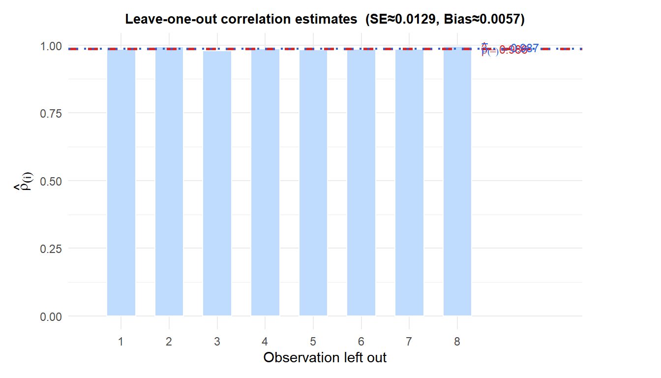
Leave-one-out estimates (bars) are all very close to the full-sample \(\hat{\rho}\) (red dashed), confirming the correlation is stable. The jackknife SE \(\approx\) 0.0129 and bias \(\approx\) 0.0057.
When the jackknife fails: non-smooth statistics
⚠️ The jackknife is inconsistent for non-smooth statistics
The jackknife is based on a linear approximation: it assumes that removing one observation changes \(\hat{\theta}\) by a small, smooth amount. For non-smooth statistics (those that can change discontinuously when one observation is added or removed) this approximation breaks down.
The classic example is the sample median with \(n\) even. Removing one observation can shift the median by a full inter-observation gap rather than a small perturbation. The jackknife variance estimate is then inconsistent: it does not converge to the true variance even as \(n \to \infty\).
Statistics for which jackknife fails or performs poorly:
- Sample median and other quantiles.
- Sample maximum and minimum.
- Number of distinct values in a sample.
- Any statistic with a discontinuity as a function of the data.
For these, use the bootstrap instead.
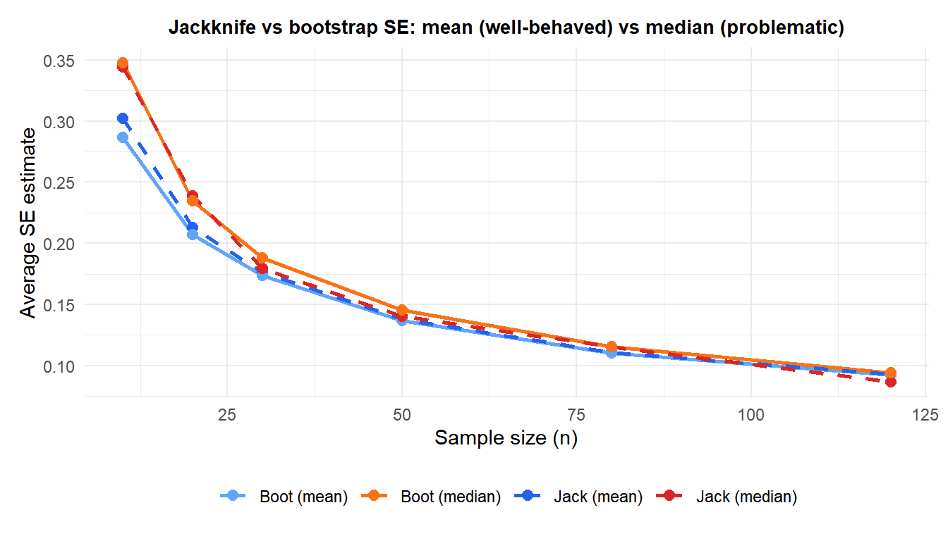
For the mean (blue tones), jackknife and bootstrap give similar SE estimates across all \(n\). For the median (red/orange), the jackknife SE (dashed red) is erratic and unreliable, while the bootstrap SE (solid orange) is consistent.
The delete-\(d\) jackknife
The standard jackknife leaves out one observation at a time. The delete-\(d\) jackknife leaves out \(d\) observations at a time, creating \(\binom{n}{d}\) subsamples. For \(d > 1\), it can handle non-smooth statistics:
\[\widehat{\text{Var}}_\text{jack-d} = \frac{\binom{n}{d}^{-1}}{n-d} \sum_{S} \left(\hat{\theta}_{(S)} - \bar{\theta}_{(\cdot)}\right)^2\]
where the sum is over all subsets \(S\) of size \(n-d\). The optimal \(d\) for non-smooth statistics satisfies \(d/n \to 1\) as \(n \to \infty\). In practice, the bootstrap is almost always preferred over delete-\(d\) jackknife for non-smooth statistics.
Jackknife vs bootstrap
| Jackknife | Bootstrap | |
|---|---|---|
| Subsamples | \(n\) (deterministic) | \(B\) (random) |
| Randomness | None | Yes (Monte Carlo) |
| Smooth statistics | Excellent | Excellent |
| Non-smooth statistics | Fails | Works |
| Computational cost | \(O(n)\) function evaluations | \(O(B \cdot n)\) |
| Bias correction | Direct formula | Requires BCa or similar |
| Historical use | Pre-1979 | Post-1979 (Efron) |
The jackknife is the bootstrap’s predecessor and remains useful for smooth statistics where its deterministic nature (no randomness, no \(B\) to choose) is an advantage. For everything else, the bootstrap is the standard tool.
💡 Jackknife in R
# Manual jackknife SE for any statistic
jackknife_se <- function(x, stat_fn) {
  n      <- length(x)
  loo    <- sapply(1:n, function(i) stat_fn(x[-i]))
  sqrt((n-1)/n * sum((loo - mean(loo))^2))
}

jackknife_se(x, mean)
jackknife_se(x, var)

# The bootstrap::jackknife() function
library(bootstrap)
jackknife(x, mean)
